
In the previous section, we discussed DBNs. In this section, we will discuss one particular variant of it, called the Hidden Markov model (HMM). Although named the Hidden Markov model, it is not a Markov network. Its etymology comes from the fact that the HMM satisfies the Markov property.
A Markov property basically indicates the memory-less property of a stochastic process, and any stochastic process satisfying this property is called as a Markov process. Let ![]() be a time-continuous process. Then, for every
be a time-continuous process. Then, for every ![]() , time points
, time points ![]() with states
with states ![]() . Then,
. Then, ![]() . This means that the current state depends only on the previous state; any additional knowledge about the history doesn't add any extra information.
. This means that the current state depends only on the previous state; any additional knowledge about the history doesn't add any extra information.
For example, if we sample the mood of a person once a minute, then it is fair to assume that the current mood of the person is only affected by his/her mood in the previous minute (unless that person is suffering from bipolar disorder). In the case of predicting the trajectory of a missile, we can also assume that the position of the missile at ![]() can be determined by
can be determined by ![]() alone. Although at first glance, this may not seem to be correct, if the trajectory is sampled very fast, it may be a very good approximation.
alone. Although at first glance, this may not seem to be correct, if the trajectory is sampled very fast, it may be a very good approximation.

Fig 7.7: Graphical model representation of a Markov process
Fig 7.7 shows the graphical model representation of a Markov process. In most applications of such models, the probability distribution ![]() is assumed to be equal for any value of t.
is assumed to be equal for any value of t. ![]() can be represented in the form of a transition matrix (A) or a state-transition diagram. For example, if we want to model the mood of a person (which can be very sad, sad, happy, or very happy), we can represent this in the form of a state-transition diagram:
can be represented in the form of a transition matrix (A) or a state-transition diagram. For example, if we want to model the mood of a person (which can be very sad, sad, happy, or very happy), we can represent this in the form of a state-transition diagram:

Fig 7.8: State-transition diagram representing the transition of the mood of a person across time
The preceding figure shows the transition of the mood of a person from one state to another. For example, from the diagram, we can infer that the probability of transitioning from a very happy state to a happy state is 0.15, the probability of remaining in the same state is 0.8, and so on. As all the edge weightings represent the probability, all the weightings corresponding to the edges outgoing from a single node should sum up to 1.
Another way of representing ![]() is with a transition matrix. A transition matrix (A) is a matrix in the shape of N x N, where N represents the number of states. Each element
is with a transition matrix. A transition matrix (A) is a matrix in the shape of N x N, where N represents the number of states. Each element ![]() of a transition matrix A represents the probability of transitioning from state
of a transition matrix A represents the probability of transitioning from state ![]() to state
to state ![]() . For example, the transition matrix corresponding to the preceding state-transition diagram would be as follows:
. For example, the transition matrix corresponding to the preceding state-transition diagram would be as follows:
|
Very Sad |
Sad |
Happy |
Very Happy | |
|---|---|---|---|---|
|
Very Sad |
0.2 |
0.6 |
0.15 |
0.05 |
|
Sad |
0.2 |
0.3 |
0.3 |
0.2 |
|
Happy |
0.05 |
0.05 |
0.7 |
0.2 |
|
Very Happy |
0.005 |
0.045 |
0.15 |
0.8 |
For the first node ![]() , there is no parent node. So unlike all other nodes, its distribution can't be encoded by the conditional probability distribution of the form
, there is no parent node. So unlike all other nodes, its distribution can't be encoded by the conditional probability distribution of the form ![]() . So, for this node, the distribution is a marginal probability distribution called the initial state probability distribution
. So, for this node, the distribution is a marginal probability distribution called the initial state probability distribution ![]() . It is an array of shape of N x 1, with the constraint
. It is an array of shape of N x 1, with the constraint ![]() . For example, in the earlier mood example, the matrix can be as follows:
. For example, in the earlier mood example, the matrix can be as follows:
|
Very Sad |
Sad |
Happy |
Very Happy |
|---|---|---|---|
|
0.1 |
0.4 |
0.4 |
0.1 |
However, in real-life situations, we can't directly observe the state of the variable, that is, the variables are hidden from us. For example, we can't observe whether a person is very sad, sad, happy, or very happy just by looking at this table. Instead, we can observe some other variable ![]() that is affected by
that is affected by ![]() . For example, the current activity of a person (which is an observable parameter) can tell us about his/her mood. Thus, the graphical model representing the system, as stated in Fig 7.7, is modified as follows:
. For example, the current activity of a person (which is an observable parameter) can tell us about his/her mood. Thus, the graphical model representing the system, as stated in Fig 7.7, is modified as follows:

Fig 7.9: Graphical model representing a Hidden Markov model
With the addition of extra nodes and edges to the graphical model, we need an additional conditional probability distribution ![]() (called emission probability), which is represented as
(called emission probability), which is represented as ![]() . It is assumed to be equal for any value of t. Thus, an HMM model can be represented by the following three parameters:
. It is assumed to be equal for any value of t. Thus, an HMM model can be represented by the following three parameters:
Thus, an HMM model can be stated as ![]() .
.
Given model ![]() , we can generate a sequence of observations
, we can generate a sequence of observations ![]() as follows:
as follows:
-
Choose an initial state
 (
( ) according to the initial state distribution
  .
.
- Set t = 1.
- Choose an observation
 corresponding to
  according to the emission probability
  .
.
- Transit to the next state
 according to the state-transition probability represented by the transition matrix A.
- Set t = t + 1 and return to step 3 if t < T, else terminate.
For HMM and its application in Python, we will use a library called hmmlearn. It is an offshoot of a popular machine learning library in Python called scikit-learn.
Let's continue with the previous mood example. Suppose we are able to observe the current activity of a person, and for the sake of simplicity, let's assume it is restricted to a few possibilities such as watching television, sleeping, eating, crying, and playing. As the observed value is also a discrete quantity, the emission probability ![]() can be represented in the form of a tabular conditional probability distribution.
can be represented in the form of a tabular conditional probability distribution.
|
Very Sad |
Sad |
Happy |
Very Happy | |
|---|---|---|---|---|
|
Watching Television |
0.045 |
0.2 |
0.3 |
0.1 |
|
Sleeping |
0.15 |
0.2 |
0.1 |
0.1 |
|
Eating |
0.2 |
0.2 |
0.1 |
0.2 |
|
Crying |
0.6 |
0.3 |
0.05 |
0.05 |
|
Playing |
0.005 |
0.1 |
0.45 |
0.55 |
The preceding distribution represents the probability given the mood of the person. For example, the first row and first column basically represent the probability of someone watching television when he/she is very sad.
To represent an HMM with multinomial (or discrete) emission, The hmmlearn library provides a class called MultinomialHMM. It's implementation in Python is as follows:
In [1]: from hmmlearn.hmm import MultinomialHMM
In [2]: import numpy as np

# Here n_components correspond to number of states in the hidden
# variables and n_symbols correspond to number of states in the
# obversed variables
In [3]: model_multinomial = MultinomialHMM(n_components=4)

# Transition probability as specified above
In [4]: transition_matrix = np.array([[0.2, 0.6, 0.15, 0.05],
                                         [0.2, 0.3, 0.3, 0.2],
                                         [0.05, 0.05, 0.7, 0.2],
                                         [0.005, 0.045, 0.15, 0.8]])
# Setting the transition probability
In [5]: model_multinomial.transmat_ = transition_matrix

# Initial state probability
In [6]: initial_state_prob = np.array([0.1, 0.4, 0.4, 0.1])

# Setting initial state probability
In [7]: model_multinomial.startprob_ = initial_state_prob

# Here the emission prob is required to be in the shape of
# (n_components, n_symbols). So instead of directly feeding the
# CPD we would using the transpose of it.
In [8]: emission_prob = np.array([[0.045, 0.15, 0.2, 0.6, 0.005],
                                  [0.2, 0.2, 0.2, 0.3, 0.1],
                                  [0.3, 0.1, 0.1, 0.05, 0.45],
                                     [0.1, 0.1, 0.2, 0.05, 0.55]])

# Setting the emission probability
In [9]: model_multinomial.emissionprob_ = emission_prob

# model.sample returns both observations as well as hidden states
# the first return argument being the observation and the second
# being the hidden states
In [10]: Z, X = model_multinomial.sample(100)
The other type of HMM model that implements in hmmlearn is GaussianHMM. It represents HMM with Gaussian emissions. Thus, for characterizing the emission probability ![]() , instead of using a complete tabular CPD, we can just provide the mean and covariance. For example, let's try to sample observations from an HMM with N = 3 and with a mean
, instead of using a complete tabular CPD, we can just provide the mean and covariance. For example, let's try to sample observations from an HMM with N = 3 and with a mean ![]() and covariance
and covariance ![]() :
:
In [1]: from hmmlearn.hmm import GaussianHMM
In [2]: import matplotlib.pyplot as plt
In [3]: import numpy as np

# Here n_components correspond to number of states in the hidden
# variables.
In [4]: model_gaussian = GaussianHMM(n_components=3,
                                     covariance_type='full')

# Transition probability as specified above
In [5]: transition_matrix = np.array([[0.2, 0.6, 0.2],
                                      [0.4, 0.3, 0.3],
                                      [0.05, 0.05, 0.9]])

# Setting the transition probability
In [6]: model_gaussian.transmat_ = transition_matrix

# Initial state probability
In [7]: initial_state_prob = np.array([0.1, 0.4, 0.5])

# Setting initial state probability
In [8]: model_gaussian.startprob_ = initial_state_prob

# As we want to have a 2-D gaussian distribution the mean has to
# be in the shape of (n_components, 2)
In [9]: mean = np.array([[0.0, 0.0],
                         [0.0, 10.0],
                         [10.0, 0.0]])

# Setting the mean
In [10]: model_gaussian.means_ = mean

# As emission probability is a 2-D gaussian distribution, thus
# covariance matrix for each state would be a 2-D matrix, thus
# overall the covariance matrix for all the states would be in the # form of (n_components, 2, 2)
In [11]: covariance = 0.5 * np.tile(np.identity(2), (3, 1, 1))
In [12]: model_gaussian.covars_ = covariance

# model.sample returns both observations as well as hidden states
# the first return argument being the observation and the second
# being the hidden states
In [13]: Z, X = model_gaussian.sample(100)

# Plotting the observations
In [14]: plt.plot(Z[:, 0], Z[:, 1], "-o", label="observations",
                  ms=6, mfc="orange", alpha=0.7)

# Indicate the state numbers
In [15]: for i, m in enumerate(mean):
             plt.text(m[0], m[1], 'Component %i' % (i + 1),
                      size=17, horizontalalignment='center',
                      bbox=dict(alpha=.7, facecolor='w'))

In [16]: plt.legend(loc='best')
In [17]: plt.show()
Fig 7.10: Plot showing 100 samples drawn from the previously stated HMM. The lines connect the successive observations.
Fig 7.10 shows the successive observations drawn from the HMM stated earlier. In this HMM, the initial state probability distribution favors the state ![]() as compared to the other two states. According to the transition matrix, the probability of transitioning state
as compared to the other two states. According to the transition matrix, the probability of transitioning state ![]() to
to ![]() is much higher as compared to transitioning from
is much higher as compared to transitioning from ![]() to any other state. Thus, we can see that most of the observations correspond to the state
to any other state. Thus, we can see that most of the observations correspond to the state ![]() as compared to any other state.
as compared to any other state.
The next problem that we are going to tackle in the case of the HMM is computing the probability of observation given a model that is computing ![]() .
.
Let's start with a simple example of an HMM with a multinomial emission (that is, the observation variable being discrete quantities). In this case, the emission probability ![]() can be represented by a matrix B such that each element
can be represented by a matrix B such that each element ![]() equals the following:
equals the following:

Here, N represents the number of possible states of a hidden variable and M represents the number of possible states of an observed variable.
Suppose ![]() is the sequence of states of the hidden variable. To compute the value of
is the sequence of states of the hidden variable. To compute the value of ![]() , we can marginalize the distribution
, we can marginalize the distribution ![]() with respect to X:
with respect to X:

Let's first compute the term ![]() . The
. The ![]() term is nothing but
term is nothing but ![]() , because given a model
, because given a model ![]() ,
, ![]() only depends on
only depends on ![]() . The
. The ![]() term can be computed as follows:
term can be computed as follows:

The ![]() term can be computed directly from the initial state probability distribution and transition matrix as follows:
term can be computed directly from the initial state probability distribution and transition matrix as follows:

Thus, ![]() can be stated in the following way:
can be stated in the following way:
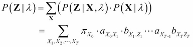
The computation of ![]() using the preceding equation requires an exponentially large number of mathematical operations, precisely
using the preceding equation requires an exponentially large number of mathematical operations, precisely ![]() multiplications and
multiplications and ![]() additions. Even for a very small value of T (for example, 100) and N as 5, it requires
additions. Even for a very small value of T (for example, 100) and N as 5, it requires ![]() operations. Thus, we require a more efficient way to compute
operations. Thus, we require a more efficient way to compute ![]() . One such method is the forward-backward algorithm.
. One such method is the forward-backward algorithm.
Before going into the details of the algorithm, let's define some variables that are needed for this routine, the first one being the forward variable ![]() . It is defined as follows:
. It is defined as follows:
The forward variable is the probability of a partially observed sequence ![]() (until a time t) and the state
(until a time t) and the state ![]() at time t, given the model
at time t, given the model ![]() .
. ![]() , can be computed inductively as the following initialization:
, can be computed inductively as the following initialization:
Here, ![]() represents the initial probability for the state
represents the initial probability for the state ![]() and
and ![]() represents the probability of
represents the probability of ![]() given the state of
given the state of ![]() .
.
The induction step:

Here, ![]() represents the probability of transitioning from the state
represents the probability of transitioning from the state ![]() to the state
to the state ![]() and
and ![]() represents the probability of
represents the probability of ![]() given
given ![]() .
.
The termination step:

The induction step is the core of the computational method.

Fig 7.11: Computation of ![]() as shown in the induction step
as shown in the induction step
Fig 7.11 shows the computation algorithm used in the induction step. The values of all the ![]() instances are weight-summed, where the weightings represent the probability of transitioning from the state
instances are weight-summed, where the weightings represent the probability of transitioning from the state ![]() to the state
to the state ![]() .
.

Fig 7.12: Implementation of the computation of ![]() in terms of the lattice of observation t and states i
in terms of the lattice of observation t and states i
This operation only requires ![]() operations, as opposed to the
operations, as opposed to the ![]() operations required by the direct calculation. So, in the case of N = 5 and T = 100, we only require 3000 computations.
operations required by the direct calculation. So, in the case of N = 5 and T = 100, we only require 3000 computations.
In a similar manner, we can use a backward pass to compute the backward variable ![]() . This is defined as follows:
. This is defined as follows:
The initialization step:
The induction step:

The hmmlearn module facilitates the computation of ![]() . For example, let's take the previously stated example of the
. For example, let's take the previously stated example of the GaussianHMM model:
# mean of the emission probability distribution for various states
# were:
# [0.0, 0.0],
# [0.0, 10.0],
# [10.0, 0.0]

# So if an observations are sampled from some other gaussian
# distribution with mean centered at different location such as:
# [5, 5]
# [-5, 0]
# the probability of these observations coming from this model
# should be very low.

# generating observations
In [18]: observations = np.row_stack((
                           np.random.multivariate_normal(
                             [5, 5], [[0.5, 0], [0, 0.5]], 10),
                           np.random.multivariate_normal(
                             [-5, 0], [[0.5, 0], [0, 0.5]], 10)))

# model.score returns the log-probability of P(observations |
# model)
In [19]: score_1 = model_gaussian.score(observations)
In [20]: print(score_1)
-728.50717880180241

# Lets try to check whether observations sampled from the
# multivariate normal distributions that were used in our HMM
# model provides greater value of score or not
In [21]: observations = np.row_stack((
                            np.random.multivariate_normal(
                               [10, 0], [[0.5, 0], [0, 0.5]], 10),
                            np.random.multivariate_normal(
                               [0, 0], [[0.5, 0], [0, 0.5]], 2),
                            np.random.multivariate_normal(
                               [0, 10], [[0.5, 0], [0, 0.5]], 4)))
In [22]: score_2 = model_gaussian.score(observations)
In [23]: print(score_2)
-44.709532774805481

# We can see that results matches our intuitionApart from computing ![]() , the other major challenges in the case of the HMM (given an observation sequence
, the other major challenges in the case of the HMM (given an observation sequence ![]() and a model
and a model ![]() ) is computing the state sequence
) is computing the state sequence ![]() that best explains the model. A single best-state sequence is defined as the state sequence X that maximizes
that best explains the model. A single best-state sequence is defined as the state sequence X that maximizes ![]() , which is equivalent to maximizing
, which is equivalent to maximizing ![]() .
.
The Viterbi algorithm is a dynamic programming-based algorithm used to compute the best-state sequence. Before going into the details of the algorithm, let's define a quantity ![]() as the best score along a single-state sequence at time t, which accounts for the first t observations and ends in the state
as the best score along a single-state sequence at time t, which accounts for the first t observations and ends in the state ![]() . This can be defined as follows:
. This can be defined as follows:
By the induction, we have the following:
To actually retrieve a state sequence, we need to keep track of the argument that is maximized for each t and j using the array ![]() . The complete procedure is as follows:
. The complete procedure is as follows:
The initialization step:

The recursion step:


The termination step:
The state sequence backtracking step:
This method is similar to what we discussed in the case of forward calculations, except for a few minor changes such as the inclusion of a backtracking step and maximization over previous states instead of summation.
The hmmlearn module also facilitates the computation of a state sequence. For example, using the previously defined HMM model with a multinomial emission:
# creating a set of random observations
# As the observations can be one of the 5 states that is [0, 4],
# we can create them using np.random.randint
In [24]: random_walk = np.random.randint(low=0, high=5, size=50)

# the array should be in the form of (n_observations, n_features)
# reshaping the array
In [25]: random_walk = random_walk[:, np.newaxis]

# model.decode finds the most likely state sequence corresponding
# to the observation. By default it uses Viterbi algorithm
# it returns 2 parameters, the first one being log probability of
# the maximum likelihood path through the HMM and second being the
# state sequence.
In [26]: logprob, state_sequence = model_multinomial.decode(
                                                 random_walk)
The next major problem in HMM is to compute the model parameters given the observations. The details of the algorithm are beyond the scope of this book, but we will provide an example of its implementation using hmmlearn.
Note
To train an HMM or to compute its model parameters, hmmlearn has a fit method in all the HMM classes. The input is a list of the sequence of the observed value. As the expectation-maximization (EM) algorithm, which is used to compute the model parameters, is a gradient-based optimization method, it will generally get stuck in a local optima. One workaround is to try the fit method with various initializations and select the highest scoring model.
In [1]: from __future__ import print_function

In [2]: import datetime
In [3]: import numpy as np
In [4]: import matplotlib.pyplot as plt
In [5]: from matplotlib.finance import quotes_historical_yahoo
In [6]: from matplotlib.dates import YearLocator, MonthLocator, DateFormatter
In [7]: from hmmlearn.hmm import GaussianHMM

# Downloading the data
In [8]: date1 = datetime.date(1995, 1, 1)  # start date
In [9]: date2 = datetime.date(2012, 1, 6)  # end date

# get quotes from yahoo finance
In [10]: quotes = quotes_historical_yahoo("INTC", date1, date2)

# unpack quotes
In [11]: dates = np.array([q[0] for q in quotes], dtype=int)
In [12]: close_v = np.array([q[2] for q in quotes])
In [13]: volume = np.array([q[5] for q in quotes])[1:]

# take diff of close value
# this makes len(diff) = len(close_t) - 1
# therefore, others quantity also need to be shifted
In [14]: diff = close_v[1:] - close_v[:-1]
In [15]: dates = dates[1:]
In [16]: close_v = close_v[1:]

# pack diff and volume for training
In [17]: X = np.column_stack([diff, volume])

# Run Gaussian HMM
In [18]: n_components = 5

# make an HMM instance and execute fit
In [19]: model = GaussianHMM(n_components, covariance_type="diag",
                             n_iter=1000)

In [20]: model.fit([X])

# predict the optimal sequence of internal hidden state
In [21]: hidden_states = model.predict(X)

# print trained parameters and plot
In [22]: print("Transition matrix")
In [23]: print(model.transmat_)

In [24]: for i in range(n_components):
             print("%dth hidden state" % i)
             print("mean = ", model.means_[i])
             print("var = ", np.diag(model.covars_[i]))

In [25]: years = YearLocator()   # every year
In [26]: months = MonthLocator()  # every month
In [27]: yearsFmt = DateFormatter('%Y')
In [28]: fig = plt.figure()
In [29]: ax = fig.add_subplot(111)

In [30]: for i in range(n_components):
         # use fancy indexing to plot data in each state
             idx = (hidden_states == i)
             ax.plot_date(dates[idx], close_v[idx], 'o',
                          label="%dth hidden state" % i)
             ax.legend()

# format the ticks
In [31]: ax.xaxis.set_major_locator(years)
In [32]: ax.xaxis.set_major_formatter(yearsFmt)
In [33]: ax.xaxis.set_minor_locator(months)
In [34]: ax.autoscale_view()

# format the coords message box
In [35]: ax.fmt_xdata = DateFormatter('%Y-%m-%d')
In [36]: ax.fmt_ydata = lambda x: '$%1.2f' % x
In [37]: ax.grid(True)
In [38]: ax.set_xlabel('Year')
In [39]: ax.set_ylabel('Closing Volume')

In [40]: fig.autofmt_xdate()
In [41]: plt.show()
Fig 7.13: Plot showing the closing volume for each of the hidden states across time. It is the output of the previously stated code.