During the learning process, it is important to design how the training should be performed. Two basic approaches are batch and incremental learning.
In batch learning, all the records are fed to the network, so it can evaluate the error and then update the weights:

In incremental learning, the update is performed after each record has been sent to the network:

Both approaches work well and have advantages and disadvantages. While batch learning can used for a less frequent, though more directed, weight update, incremental learning provides a method for fine-tuned weight adjustment. In that context, it is possible to design a mode of learning that enables the network to learn continually.
Offline learning means that the neural network learns while not in operation. Every neural network application is supposed to work in an environment, and in order to be at production, it should be properly trained. Offline training is suitable for putting the network into operation, since its outputs may be varied over large ranges of values, which would certainly compromise the system, if it is in operation. But when it comes to online learning, there are restrictions. While in offline learning, it's possible to use cross-validation and bootstrapping to predict errors, in online learning, this can't be done since there's no "training dataset" anymore. However, one would need online training when some improvement in the neural network's performance is desired.
A stochastic method is used when online learning is performed. This algorithm to improve neural network training is composed of two main features: random choice of samples for training and variation of learning rate in runtime (online). This training method has been used when noise is found in the objective function. It helps to escape the local minimum (one of the best solutions) and to reach the global minimum (the best solution):
The pseudo-algorithm is displayed below (source: ftp://ftp.sas.com/pub/neural/FAQ2.html#A_styles):
Initialize the weights.
   Initialize the learning rate.
   Repeat the following steps:
      Randomly select one (or possibly more) case(s)
         from the population.
      Update the weights by subtracting the gradient
         times the learning rate.
      Reduce the learning rate according to an
appropriate schedule.The Java project has created the class BackpropagtionOnline inside the learn package. The differences between this algorithm and classic Backpropagation was programmed by changing the train() method, by adding two new methods: generateIndexRandomList() and reduceLearningRate(). The first one generates a random list of indexes to be used in the training step and the second one executes the learning rate online variation according to the following heuristic:
private double reduceLearningRate(NeuralNet n, double percentage) {
    double newLearningRate = n.getLearningRate() *
                    ((100.0 - percentage) / 100.0);

    if(newLearningRate < 0.1) {
      newLearningRate = 1.0;
    }

    return newLearningRate;
  }
This method will be called at the end of the train() method.
It has used data from previous chapters to test this new way to train neural nets. The same neural net topology defined in each chapter (Chapter 5, Forecasting Weather and Chapter 8, Text Recognition) has been used to train the nets of this chapter. The first one is the weather forecasting problem and the second one is the OCR. The following table shows the comparison of results:

In addition, charts of the MSE evolution have been plotted and are shown here:
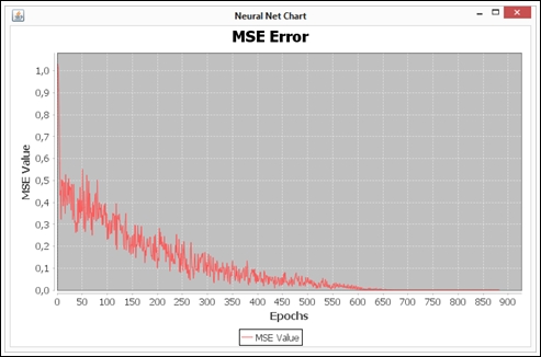

The curve showed in the first chart (Weather Forecast) has a saw shape, because of the variation of learning rate. Besides, it's very similar to the curve, as shown in Chapter 5, Forecasting Weather On the other hand, the second chart (OCR) shows that the training process was faster and stops near the 900th epoch because it reached a very small MSE error.
Other experiments were made: training neural nets with a backpropagation algorithm, and considering the learning rate found by the online approach. The MSE values reduced in both problems:

Another important observation consists in the fact that training process demonstrated by the training terminated almost in the 3,000th epoch. Therefore, it's faster and better than the training process seen in Chapter 8, Text Recognition using the same algorithm.