If there's a problem with the network being tied densely, just force it to be sparse. Then the vanishing gradient problem won't occur and learning can be done properly. The algorithm based on such an idea is the dropout algorithm. Dropout for deep neural networks was introduced in Improving neural networks by preventing co adaptation of feature detectors (Hinton, et. al. 2012, http://arxiv.org/pdf/1207.0580.pdf) and refined in Dropout: A Simple Way to Prevent Neural Networks from Overfitting (Srivastava, et. al. 2014, https://www.cs.toronto.edu/~hinton/absps/JMLRdropout.pdf). In dropout, some of the units are, literally, forcibly dropped while training. What does this mean? Let's look at the following figures—firstly, neural networks:

There is nothing special about this figure. It is a standard neural network with one input layer, two hidden layers, and one output layer. Secondly, the graphical model can be represented as follows by applying dropout to this network:

Units that are dropped from the network are depicted with cross signs. As you can see in the preceding figure, dropped units are interpreted as non-existent in the network. This means we need to change the structure of the original neural network while the dropout learning algorithm is being applied. Thankfully, applying dropout to the network is not difficult from a computational standpoint. You can simply build a general deep neural network first. Then the dropout learning algorithm can be applied just by adding a dropout mask—a simple binary mask—to all the units in each layer. Units with the value of 0 in the binary mask are the ones that are dropped from the network.

This may remind you of DA (or SDA) discussed in the previous chapter because DA and dropout look similar at first glance. Corrupting input data in DA also adds binary masks to the data when implemented. However, there are two remarkably different points between them. First, while it is true that both methods have the process of adding masks to neurons, DA applies the mask only to units in the input layer, whereas dropout applies it to units in the hidden layer. Some of the dropout algorithms apply masks to both the input layer and the hidden layer, but this is still different from DA. Second, in DA, once the corrupt input data is generated, the data will be used throughout the whole training epochs, but in dropout, the data with different masks will be used in each training epoch. This indicates that a neural network of a different shape is trained in each iteration. Dropout masks will be generated in each layer in each iteration according to the probability of dropout.

You might have a question—can we train the model even if the shape of the network is different in every step? The answer is yes. You can think of it this way—the network is well trained with dropout because it puts more weights on the existing neurons to reflect the characteristics of the input data. However, dropout has a single demerit, that is, it requires more training epochs than other algorithms to train and optimize the model, which means it takes more time until it is optimized. Another technique is introduced here to reduce this problem. Although the dropout algorithm itself was invented earlier, it was not enough for deep neural networks to gain the ability to generalize and get high precision rates just by using this method. With one more technique that makes the network even more sparse, we achieve deep neural networks to get higher accuracy. This technique is the improvement of the activation function, which we can say is a simple yet elegant solution.

All of the methods of neural networks explained so far utilize the sigmoid function or hyperbolic tangent as an activation function. You might get great results with these functions. However, as you can see from the shape of them, these curves saturate and kill the gradients when the input values or error values at a certain layer are relatively large or small.

One of the activation functions introduced to solve this problem is the rectifier. A unit-applied rectifier is called a Rectified Linear Unit (ReLU). We can call the activation function itself ReLU. This function is described in the following equation:

The function can be represented by the following figure:

The broken line in the figure is the function called a softplus function, the derivative of it is logistic function, which can be described as follows:

This is just for your information: we have the following relations that a smooth approximation to the rectifier. As you can see from the figure above, since the rectifier is far simpler than the sigmoid function and hyperbolic tangent, you can easily guess that the time cost will reduce when it is applied to the deep learning algorithm. In addition, because the derivative of the rectifier—which is necessary when calculating backpropagation errors—is also simple, we can, additionally, shorten the time cost. The equation of the derivative can be represented as follows:

Since both the rectifier and the derivative of it are very sparse, we can easily imagine that the neural networks will be also sparse through training. You may have also noticed that we no longer have to worry about gradient saturations because we don't have the causal curves that the sigmoid function and hyperbolic tangent contain anymore.

With the technique of dropout and the rectifier, a simple deep neural network can learn a problem without pre-training. In terms of the equations used to implement the dropout algorithm, they are not difficult because they are just simple methods of adding dropout masks to multi-layer perceptrons. Let's look at them in order:

Here, denotes the activation function, which is, in this case, the rectifier. You see, the previous equation is for units in the hidden layer without dropout. What the dropout does is just apply the mask to them. It can be represented as follows:

Here, denotes the probability of dropout, which is generally set to 0.5. That's all for forward activation. As you can see from the equations, the term of the binary mask is the only difference from the ones of general neural networks. In addition, during backpropagation, we also have to add masks to the delta. Suppose we have the following equation:

With this, we can define the delta as follows:

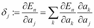
Here, denotes the evaluation function (these equations are the same as we mentioned in Chapter 2, Algorithms for Machine Learning – Preparing for Deep Learning). We get the following equation:

Here, the delta can be described as follows:

Now we have all the equations necessary for implementation, let's dive into the implementation. The package structure is as follows:

First, what we need to have is the rectifier. Like other activation functions, we implement it in ActivationFunction.java as ReLU:

public static double ReLU(double x) {
   if(x > 0) {
       return x;
   } else {
       return 0.;
   }
}

Also, we define dReLU as the derivative of the rectifier:

public static double dReLU(double y) {
   if(y > 0) {
       return 1.;
   } else {
       return 0.;
   }
}

Accordingly, we updated the constructor of HiddenLayer.java to support ReLU:

if (activation == "sigmoid" || activation == null) {

   this.activation = (double x) -> sigmoid(x);
   this.dactivation = (double x) -> dsigmoid(x);

} else if (activation == "tanh") {

   this.activation = (double x) -> tanh(x);
   this.dactivation = (double x) -> dtanh(x);

} else if (activation == "ReLU") {

   this.activation = (double x) -> ReLU(x);
   this.dactivation = (double x) -> dReLU(x);

} else {
   throw new IllegalArgumentException("activation function not supported");
}

Now let's have a look at Dropout.java. In the source code, we'll build the neural networks of two hidden layers, and the probability of dropout is set to 0.5:

int[] hiddenLayerSizes = {100, 80};
double pDropout = 0.5;

The constructor of Dropout.java can be written as follows (since the network is just a simple deep neural network, the code is also simple):

public Dropout(int nIn, int[] hiddenLayerSizes, int nOut, Random rng, String activation) {

   if (rng == null) rng = new Random(1234);

   if (activation == null) activation = "ReLU";

   this.nIn = nIn;
   this.hiddenLayerSizes = hiddenLayerSizes;
   this.nOut = nOut;
   this.nLayers = hiddenLayerSizes.length;
   this.hiddenLayers = new HiddenLayer[nLayers];
   this.rng = rng;

   // construct multi-layer
   for (int i = 0; i < nLayers; i++) {
       int nIn_;
       if (i == 0) nIn_ = nIn;
       else nIn_ = hiddenLayerSizes[i - 1];

       // construct hidden layer
       hiddenLayers[i] = new HiddenLayer(nIn_, hiddenLayerSizes[i], null, null, rng, activation);
   }

   // construct logistic layer
   logisticLayer = new LogisticRegression(hiddenLayerSizes[nLayers - 1], nOut);
}

As explained, now we have the HiddenLayer class with ReLU support, we can use ReLU as the activation function.

Once a model is built, what we do next is train the model with dropout. The method for training is simply called train. Since we need some layer inputs when calculating the backpropagation errors, we define the variable called layerInputs first to cache their respective input values:

List<double[][]> layerInputs = new ArrayList<>(nLayers+1);
layerInputs.add(X);

Here, X is the original training data. We also need to cache the dropout masks for each layer for backpropagation, so let's define it as dropoutMasks:

List<int[][]> dropoutMasks = new ArrayList<>(nLayers);

Training begins in a forward activation fashion. Look how we apply the dropout masks to the value; we merely multiply the activated values and binary masks:

// forward hidden layers
for (int layer = 0; layer < nLayers; layer++) {

   double[] x_;  // layer input
   double[][] Z_ = new double[minibatchSize][hiddenLayerSizes[layer]];
   int[][] mask_ = new int[minibatchSize][hiddenLayerSizes[layer]];

   for (int n = 0; n < minibatchSize; n++) {

       if (layer == 0) {
           x_ = X[n];
       } else {
           x_ = Z[n];
       }


       Z_[n] = hiddenLayers[layer].forward(x_);
       mask_[n] = dropout(Z_[n], pDrouput);  // apply dropout mask to units
   }

   Z = Z_;
   layerInputs.add(Z.clone());

   dropoutMasks.add(mask_);
}

The dropout method is defined in Dropout.java as well. As explained in the equation, this method returns the values following the Bernoulli distribution:

public int[] dropout(double[] z, double p) {

   int size = z.length;
   int[] mask = new int[size];

   for (int i = 0; i < size; i++) {
       mask[i] = binomial(1, 1 - p, rng);
       z[i] *= mask[i]; // apply mask
   }

   return mask;
}

After forward propagation through the hidden layers, training data is forward propagated in the output layer of the logistic regression. Then, in the same way as the other neural networks algorithm, the deltas of each layer are going back through the network. Here, we apply the cached masks to the delta so that its values are backpropagated in the same network:

// forward & backward output layer
D = logisticLayer.train(Z, T, minibatchSize, learningRate);

// backward hidden layers
for (int layer = nLayers - 1; layer >= 0; layer--) {

   double[][] Wprev_;

   if (layer == nLayers - 1) {
       Wprev_ = logisticLayer.W;
   } else {
       Wprev_ = hiddenLayers[layer+1].W;
   }

   // apply mask to delta as well
   for (int n = 0; n < minibatchSize; n++) {
       int[] mask_ = dropoutMasks.get(layer)[n];

       for (int j = 0; j < D[n].length; j++) {
           D[n][j] *= mask_[j];
       }
   }

   D = hiddenLayers[layer].backward(layerInputs.get(layer), layerInputs.get(layer+1), D, Wprev_, minibatchSize, learningRate);
}

After the training comes the test phase. But before we apply the test data to the tuned model, we need to configure the weights of the network. Dropout masks can't be simply applied to the test data because when masked, the shape of each network will be differentiated, and this may return different results because a certain unit may have a significant effect on certain features. Instead, what we do is smooth the weights of the network, which means we simulate the network where whole units are equally masked. This can be done using the following equation:

As you can see from the equation, all the weights are multiplied by the probability of non-dropout. We define the method for this as pretest:

public void pretest(double pDropout) {

   for (int layer = 0; layer < nLayers; layer++) {

       int nIn_, nOut_;

       if (layer == 0) {
           nIn_ = nIn;
       } else {
           nIn_ = hiddenLayerSizes[layer];
       }

       if (layer == nLayers - 1) {
           nOut_ = nOut;
       } else {
           nOut_ = hiddenLayerSizes[layer+1];
       }

       for (int j = 0; j < nOut_; j++) {
           for (int i = 0; i < nIn_; i++) {
               hiddenLayers[layer].W[j][i] *= 1 - pDropout;
           }
       }
   }
}

We have to call this method once before the test. Since the network is a general multi-layered neural network, what we need to do for the prediction is just perform forward activation through the network:

public Integer[] predict(double[] x) {

   double[] z = new double[0];

   for (int layer = 0; layer < nLayers; layer++) {

       double[] x_;

       if (layer == 0) {
           x_ = x;
       } else {
           x_ = z.clone();
       }

       z = hiddenLayers[layer].forward(x_);
   }

   return logisticLayer.predict(z);
}

Compared to DBN and SDA, the dropout MLP is far simpler and easier to implement. It suggests the possibility that with a mixture of two or more techniques, we can get higher precision.