
2
Variational Methods for Algebraic Equations
Let us begin our exploration of variational methods by a situation which may appear as simple, but contains the fundamental elements necessary to the implementation of variational methods in complex situations: the variational formulation of algebraic equations and its consequences.
Indeed, the fundamental variational standpoint consists of no more saying that x = 0, but that x ∈ ![]() and xy = 0, ∀y ∈
and xy = 0, ∀y ∈ ![]() .
.
The apparent simplicity of this fundamental change of viewpoint masks a radical transformation in the way of thinking, having profound consequences, which can be measured by the progress performed in engineering with the help of variational tools such as analytical mechanics, hamiltonian mechanics, control theory and modern numerical methods such as finite elements, finite volumes, spectral methods, particle methods and others.
Let us illustrate these consequences by adopting the variational point of view when studying a system of algebraic equations: for instance, let us consider;
and the algebraic equations;
The variational formulation of this system of algebraic equations reads as:
An alternative variational formulation is given by:
All these formulations are equivalent:
For m < n, the equations are under-determined (less equations than unknowns); for m > n, the equations are over-determined (more equations than unknowns). This classification does not imply the existence or nonexistence of solutions.
2.1. Linear systems
Let us consider a full rank matrix A having dimensions n × n and a column matrix B having dimensions n × 1. The linear system AX = B corresponds to the particular situation where,
and we have m = n. The variational formulation is:
Assume that we are interested in the single value of x1: let us denote by A(:,j) the j-th column of A and by A(:,2:n) the matrix formed by the columns 2 to n of A:

When
we have:
and
which determines x1. This idea can be directly generalized to the situation where the variables are separated in two disjoined lists J = {j1,…,jnj] and K = {1,…,n} − {j1,…,jn} = {k1,…,kn−nj}. If we are interested in the single values of the nj variables corresponding to the indexes J, we may consider:

and
For
we have:
and
This equality involves only the variables xJ: for convenient choices of y, it furnishes an nj × nj linear system for the nj unknowns xJ.
EXAMPLE 2.1.– Let us consider the linear system
Taking y = (2 − 1)t, we have:
Using y = (−1 2)t, we have;
![]()
EXAMPLE 2.2.– Let us consider the system shown in Figure 2.1.

Figure 2.1. A physical interpretation of the method
The forces on the springs are, respectively, k1u1, k2(u2 − u1), k3(u3 − u2), so that the equilibrium of the system reads as:

what corresponds to the linear system AU = B, with
Assume that the force f is known and the displacements at the equilibrium ui of each mass mi have been measured. We are interested in determining the values of ki. Taking y = (1 1 1)t, we have:
Using y = (0 1 1)t, we have:
Using y = (0 0 1)t, we have:
Each one of the preceding choices leads to the determination of one of the values of ki. These choices may be interpreted in terms of a physical quantity: the work of the springs’ forces for a given displacement: for each displacement y, the work of two of the springs’ forces is equal to zero, while the remaining one is different from zero. In terms of virtual works, each displacement makes work a single spring, what lead to the determination of its stiffness. For instance, the displacements y = (1 1 1)t correspond to an equal displacement of all the masses. In this case, only the first spring is under tension. Analogously, y = (0 1 1)t keeps the first and the third springs without tension. Finally, y = (0 0 1)t makes that the single third spring is under tension. This approach extends to more complex linear systems (see, for instance, [GRE 89]).
![]()
In practice, the vectors y have to be chosen in order to verify ytAk = 0. They may be determined by Gauss pivoting and operations on lines. For instance, we may use the program


Program 2.1. A class for the determination of partial solutions of linear systems
This class contains a method partial_solution which determines the values of the unknowns given in list_unknowns without determining the values of the other unknowns. For instance, the code:
n = 100;
% size of the system
a = randn(n,n);
% generates a gaussian distributed random matrix
b = rand(n,1);
% generates a uniformly distributed random second member
ls = linear_system(a,b);
xsol = ls.complete_solution();
% find the exact solution
list_unknowns = [1 fix(n/10) fix(n/2)];
% unknowns to be determined
tol_zero = 1e-10;
% numerical value of zero
x = ls.partial_solution(list_unknowns, tol_zero);
% solution
err_abs = norm(x(list_unknowns)- xsol(list_unknowns));
err_rel = err/norm(xsol(list_unknowns));
% comparison complete/partial
produces err_abs =3.2601e−15, err_rel =4.8700e− 15, which corresponds to a relative error of 1e-11 %. Since the matrices are random, each run produces a different result. For instance, a second run produces err_abs =5.6125e-15, err_rel =5.0186e-15, which corresponds to a relative error of 1e-l2 %. The user will have different results, due to randomness in the definition of the matrices.
2.2. Algebraic equations depending upon a parameter
Let us consider the system of algebraic equations:
where F: ![]() n × (a, b) →
n × (a, b) → ![]() m, F = (F1, …, Fm)t Fj:
m, F = (F1, …, Fm)t Fj: ![]() n × (a, b) →
n × (a, b) → ![]() , for 1 ≤ i ≤ and t is a real parameter. Since the equations depend upon t, the solution x depends on t: x = x(t) and it is more appropriate to write
, for 1 ≤ i ≤ and t is a real parameter. Since the equations depend upon t, the solution x depends on t: x = x(t) and it is more appropriate to write
The variational formulation of this system of algebraic equations may be formulated as:
A practical way in order to eliminate the parameter t is to consider = y(t):
and integrate this last equation on (a, b):
As in the standard situation, an alternative variational formulation is given by:
Here yet, a practical way in order to eliminate the parameter t is to consider yi = yi(t):
and integrate this equation on (a, b):
As in the standard situation, all these formulations are equivalent:
2.2.1. Approximation of the solution by collocation
For engineers, a practical question concerns the determination of approximate solutions. For instance, the solution may be determined at some particular values of t – for instance, t1,…,tns – leading to particular values of y− for instance, x1,…,xns – and an interpolation may be performed in order to generate values for arbitrary t. This approach is usually referred to as collocation. In practice, it involves a family of interpolation functions
such as, for instance, φi(t) = ti−1 (polynomial interpolation). Then, an approximation:
is determined by solving the linear system of algebraic equations:
The unknowns to be determined are the coefficients up ∈ ![]() n, for p = 1, … k. They can be arranged in a matrix
n, for p = 1, … k. They can be arranged in a matrix ![]() such that upj = (up)j However, the data xr ∈
such that upj = (up)j However, the data xr ∈ ![]() n may be arranged in a matrix
n may be arranged in a matrix ![]() such that xri = (xr)i, so that these equations read as:
such that xri = (xr)i, so that these equations read as:
where, for 1 ≤ i,j ≤ n, 1≤ p ≤ k, 1≤ r ≤ ns,
These equations may be transformed in a standard linear system involving two indexes by using the transformation.
By setting I = index(r, i, ns), J = index(p, j, k), ![]() ,
, ![]() ,
, ![]() , we have
, we have ![]() . This linear system has dimension n.ns × k.n. For ns > k, it is overdetermined and least squares solution may be used – under Matlab®, this is made automatically. Notice that it may also be solved component by component: let us introduce:
. This linear system has dimension n.ns × k.n. For ns > k, it is overdetermined and least squares solution may be used – under Matlab®, this is made automatically. Notice that it may also be solved component by component: let us introduce:
Then, for 1 ≤ i ≤ n,
Thus, the solution may be sequentially determined by solving n linear systems of size ns × k.
2.2.2. Variational approximation of the solution
Collocation may be sensitive to errors in the numerical determination of x1, … xns. The variational formulations presented furnish a more robust method for the determination of the solution.
By denoting Φ = (φ1, … ,φk)t, we have x ≈ UtΦ. By taking yi(t) = φj(t) in equation [2.6], we obtain, for 1 ≤ i ≤ m; 1 ≤ p ≤ k.
so that;
This system contains k × m equations for k × n unknowns. When m = n, the numbers of equations and unknowns coincide For m < n, the equations are under-determined (less equations than unknowns); for m > n, the equations are over-determined (more equations than unknowns). As in the previous situation, this classification does not imply the existence or nonexistence of solutions. Equation [2.7] must be solved by an appropriated method, such as, for instance, Newton–Raphson, quasi-newton or fixed-point iterations. As an alternative, we may look for:
We observe that;
with
These equations may be invoked for the evaluation of the gradients when using optimization methods.
2.2.3. Linear equations
The particular situation where
leads to a linear system. In this case,
so that;
and
where
These equations may be transformed in a standard linear system involving two indexes by using the transformation previously introduced: I = index(p, i, k), J = index(q, j, k), ![]() ,
, ![]() ,
, ![]() . Then,
. Then, ![]() .
.
2.2.4. Connection to orthogonal projections
The variational approach may be interpreted in terms of orthogonal projection: let V be the set of all the functions defined on (a, b) and taking their values on ![]() .
.
V is a linear space (i.e. a vector space) and ![]() generates a finite dimensional subspace S ⊂ V:
generates a finite dimensional subspace S ⊂ V:
Since dim(S) = k, S may be assimilated to ![]() k: the element s = stΦ∈ S is entirely defined by the vector s = (s1,…,sk)t ∈
k: the element s = stΦ∈ S is entirely defined by the vector s = (s1,…,sk)t ∈ ![]() k. Let us consider a particular scalar product for vectors u, v ∈
k. Let us consider a particular scalar product for vectors u, v ∈ ![]() k:
k:
We have:
where = utΦ, v = vtΦ ∈ S ⊂ V. Let us extend this definition as being a scalar product on the whole space V:
Recall that u ⊥ v ⇔ (u, v) = 0, i.e. u and v; are orthogonal if and only if their scalar product is null. Let PS:V → S denote the orthogonal projection onto S. For u ∈ V, Ps(u) is characterized by (see section 3.7)
or, equivalently
Equation [2.7] shows that, for 1 ≤ i ≤ m,
So, for 1≤ i ≤ m,
Thus,
So, the orthogonal projection of Fi(UtΦ(t), t) onto S is null for 1 ≤ i ≤ m:
Let us consider the Cartesian product Sm = S × … × S (m times) We have also
Thus, the orthogonal projection of F(UtΦ(t), t) onto Sm is null:
In the particular situation where
we have, on the one hand, m = n and, on the other hand,
Thus, ![]() and, on the one hand,
and, on the one hand,
![]() is the orthogonal projection of fi onto S
is the orthogonal projection of fi onto S
while, on the other hand (recall that m = n),
![]() is the orthogonal projection of f onto Sm.
is the orthogonal projection of f onto Sm.
2.2.5. Numerical determination of the orthogonal projections
Let us consider an element u ∈ Vn and its orthogonal projection ![]() onto Sn We have:
onto Sn We have:
Thus, ![]() ,where;
,where;
So,
Analogously to collocation, these equations form a linear system for the coefficients ![]() . By setting, for 1 ≤ p, q ≤ k, 1 ≤ i, j ≤ n,
. By setting, for 1 ≤ p, q ≤ k, 1 ≤ i, j ≤ n,
we have:
These equations may be transformed in a standard linear system involving two indexes by setting I = index(q, i, k),
J = index(p, j, k), ![]() ,
, ![]() ,
, ![]() : then
: then ![]() . This linear system has dimension kn × kn. It may also be solved component by component: let us introduce:
. This linear system has dimension kn × kn. It may also be solved component by component: let us introduce:
Then, for 1 ≤ i ≤ n,
Thus, the solution may be sequentially determined by solving n linear systems of size × k.
2.2.6. Matlab® classes for a numerical solution
In order to determine numerical solutions, we need to define the family ![]() For instance, in one-dimensional (1D) situations, we may use a polynomial family defined by the following class:
For instance, in one-dimensional (1D) situations, we may use a polynomial family defined by the following class:


In this code, the polynomials are ![]() , with xmin=a and xmin= b. Property zero defines numbers which are treated as zero. degree defines the degree of the polynomial to be used. Property spmatrix is a square matrix containing the integrals of the products of the elements of the basis, while property intmatrix is a vector containing the integrals of the elements themselves.
, with xmin=a and xmin= b. Property zero defines numbers which are treated as zero. degree defines the degree of the polynomial to be used. Property spmatrix is a square matrix containing the integrals of the products of the elements of the basis, while property intmatrix is a vector containing the integrals of the elements themselves.
Let us assume that the data is given by a structure approxdata having as properties: points, values, subprogram, which contain, respectively, the points x, the corresponding values f(x) and a subprogram evaluating f(x). In this case, the coefficients of an approximation and, namely, orthogonal projections may be evaluated by using the following class:


This class contains a method approx_coefficients which determines the coefficients of the approximation according to the method chosen: ‘collocation’ uses the collocation approach, while the others use the variational approach, but differ in the manner where the integrals are evaluated: ‘variational_mean’ uses the data in order to evaluate a mean value approximation, ‘variational_int’ uses the quadrature by Matlab®, ‘variational_sp’ uses the matrix of integrals spmatrix furnished in the definition of the polynomial basis. The class also contains methods integrate and derive for the evaluation of an integral on the interval (xmin, xmax) and the derivative at a vector of points, respectively.
Let us illustrate the use of these classes. For instance, let us consider the noisy data generated as follows:
f = @(t) exp(t);
t = (-1:0.2:1);
p.x = t';
p.dim = 1;
x = spam.partition(f,p);
noise = 0.1;
td = (-1:0.05:1);
xd = spam.points('vector',f,td);
vd = (1+ noise*(2*rand(size(xd))-1)).*xd;
fnoise = @(t) interp1(td,vd,t,'linear');
data.points = p;
data.values = (1+ noise*(2*rand(size(x))-1)).*x;
data.subprogram = @(t) fnoise(t);
data.dim = 1;
These commands generate noisy data representing the exponential function on the interval (−1,1). The level of noise is 10%. Notice that the subprogram evaluating the function is not the exact exponential, but a noisy version generated by linear interpolation of noisy data. The commands
xmin = -1;
xmax = 1;
degree = 4;
zero = 1e-3;
phi = polynomial_basis(zero,xmin,xmax,degree);
b = basis(phi);
u1 = b.approx_coeffs('collocation',data);
generate the coefficients of the approximation by collocation by using a polynomial basis involving a maximal degree 4. The command

generates the coefficients corresponding to the variational approximation and evaluate the integrals by using the means. The command

generates the variational approximation and evaluates the integrals by using subprogram integration.
The results are shown in Figure 2.2 (recall that data is given on (−1,1) and points outside this interval are extrapolated ones):

Figure 2.2. Orthogonal projection in a simple noisy situation. For a color version of the figure, see www.iste.co.uk/souzadecursi/variational.zip
The derivative is shown below.
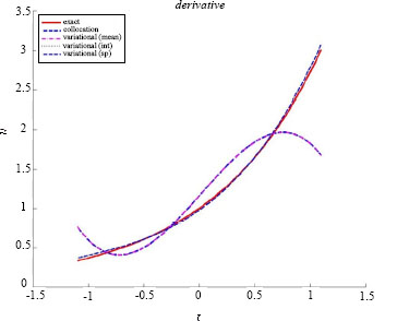
Figure 2.3. Derivative in a simple noisy situation. For a color version of the figure, see www.iste.co.uk/souzadecursi/variational.zip
We observe that, on the one hand, the results by collocation and variational approach with integrals evaluated by the mean are close and, on the other hand, the results furnished by the variational approach with more sophisticated integration are close to exact ones. Concerning the evaluation of the integral of f on the interval (−1,1), the commands
v1 = b.integrate(u1);
v2 = b.integrate(u2);
v3 = b.integrate(u3);
v4 = b.integrate(u4);
ff = @(t) b.projection(u4,t);
v5 = integral(f,-1,1);
furnish v1 = v2 = 2.3535, v3 = v4 = v5 = 2.3442, while the exact value is e − e−1≈ 2.3504.
Results for the vector (t) = (sin(πt) exp(t)t are given in Figures 2.4 and 2.5. We use a degree 5. In this situation, we obtain v1 = v2 = (−0.0139 2.3507), v3 = 0.0027 2.3658).

Figure 2.4. Orthogonal projection in a simple noisy situation. For a color version of the figure, see www.iste.co.uk/souzadecursi/variational.zip

Figure 2.5. Derivative in a simple noisy situation. For a color version of the figure, see www.iste.co.uk/souzadecursi/variational.zip
When considering nonlinear parametric equations involving a single parameter, we may use the following class


Program 2.4. Variational solution of parametric algebraic equations
In this class, the solution is obtained either by minimizing the quadratic mean square of the elements of ![]() (U) or by solving the equations
(U) or by solving the equations ![]() (U) = 0. The optimization step is performed by using the intrinsic Matlab® function fminsearch., while the determination of a zero is performed by the intrinsic function fzero. Parameters such as number of iterations, function evaluations, precision are defined by using optimset. Choice ‘mean’ evaluates the integrals by using the mean value approximation with ns equal subintervals, while ‘integral’ uses the intrinsic quadrature of Matlab®. The equations are given by structured data in equations, which has as fields subprogram, neq, dim, which correspond, respectively, to the subprogram which furnishes the value of F(x, t), the number of equations and the number of unknowns (dimension of the unknown).
(U) = 0. The optimization step is performed by using the intrinsic Matlab® function fminsearch., while the determination of a zero is performed by the intrinsic function fzero. Parameters such as number of iterations, function evaluations, precision are defined by using optimset. Choice ‘mean’ evaluates the integrals by using the mean value approximation with ns equal subintervals, while ‘integral’ uses the intrinsic quadrature of Matlab®. The equations are given by structured data in equations, which has as fields subprogram, neq, dim, which correspond, respectively, to the subprogram which furnishes the value of F(x, t), the number of equations and the number of unknowns (dimension of the unknown).
EXAMPLE 2.3.–Let us consider the simple situation where,
We use the polynomial basis with a degree 6. The code is:
xmin = 0;
xmax = pi;
ns = 500;
degree = 6;
zero = 1e-3;
phi = polynomial_basis(zero,xmin,xmax,degree);
b = basis(phi);
f = @(x,t) x - sin(t);
eqs.subprogram = f;
eqs.dim = 1;
eqs.neq = 1;
The obvious solution is x = sin(t). The results furnished by using:
pa = parametric_algebraic(eqs,b,ns);
nitmax = 10000;
U1 = pa.solve_zero('integral',U0,nitmax);
U2 = pa.solve_min('mean',U0,nitmax)
are shown in Figure 2.6 below (left: methods integral and solve_zero, right: methods mean and solve_min).
![]()

Figure 2.6. Solutions obtained for a polynomial of degree 6. For a color version of the figure, see www.iste.co.uk/souzadecursi/variational.zip
EXAMPLE 2.4.– Let us consider the simple situation where,
We use the polynomial basis with a degree 5. The code is:
xmin = 0;
xmax = pi;
ns = 500;
degree = 5;
zero = 1e-3;
phi = polynomial_basis(zero,xmin,xmax,degree);
b = basis(phi);
f = @(x,t) [x(1) + x(2) - sin(t) ; x(1) - x(2) -
cos(t)];
eqs.subprogram = f;
eqs.dim = 2;
eqs.neq = 2;
pa = parametric_algebraic(eqs,b,ns);
U1 = pa.solve_zero(
'mean',U0,nitmax);
U2 = pa.solve_min(
'integral',U0,nitmax);
The obvious solution is x1 = (sin(t) + cos (t))/2, x1 = (sin(t) − cos(t))/2. The results are shown in Figures 2.7 (using method solve_zero, integrals evaluated by the mean) and 2.8 (using method solve_min, integrals evaluated by quadrature) below.
![]()

Figure 2.7. Solutions obtained for a polynomial of degree 5 and “mean” method. For a color version of the figure, see www.iste.co.uk/souzadecursi/variational.zip

Figure 2.8. Solutions obtained for a polynomial of degree 5 and “integral” method. For a color version of the figure, see www.iste.co.uk/souzadecursi/variational.zip
EXAMPLE 2.5.– Let us consider the simple situation where
We use the polynomial basis with a degree 6. The results furnished by using method solve_zero are shown in Figure 2.9.
EXAMPLE 2.6.– Let us consider the simple situation where

Figure 2.9. Solutions obtained for a polynomial of degree 6. For a color version of the figure, see www.iste.co.uk/souzadecursi/variational.zip

Figure 2.10. Solutions obtained for a polynomial of degree 5. For a color version of the figure, see www.iste.co.uk/souzadecursi/variational.zip
We use the polynomial basis with a degree 5. The results are shown in Figure 2.10 (using method solve_zero).
![]()
Other families may be used, such as, for instance, the trigonometric family: φ1(t) = 1, φ2i(t) = cos(it) φ2i+1(t) = sin(it) or the family associated with finite elements P1. These families are defined by the classes below.


Let us illustrate the use of these classes: consider again f(x, t) = x−sin(t), what corresponds to the orthogonal projection of x = sin (t) onto the linear subspaces generated by the basis. The results are shown in the figures below. P1 Finite Elements have a piecewise constant derivative.

Figure 2.11. Solutions obtained by collocation using different basis. For a color version of the figure, see www.iste.co.uk/souzadecursi/variational.zip
2.3. Exercises
Exercise 2.1.– Consider the linear system:
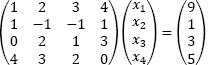
Find a vector y such that:

and determine x1 and x4 by the variational method.
![]()

Figure 2.12. Solutions obtained by variational approach (mean) using different basis. For a color version of the figure, see www.iste.co.uk/souzadecursi/variational. zip
Exercise 2.2.– Consider the linear system:

Find a vector y such that:

and determine x1 and x4 by the variational method.
Exercise 2.3.– Consider the family ψn(s) = sn−1, defined on Ω = (0,1). Denote
and the family φn(s) given by:
Show that (φn, φm) = 0 f or m < n. Conclude that (φn, φm) = 0 f or m ≠ n, so that the matrix defined by the property spmatrix is diagonal. Show that the orthogonal projection ![]() satisfies:
satisfies:
![]()
Exercise 2.4.– Consider the family φ1(t) = 1, φ2n(t) = cos(2nπt), φ2n+1(t) = sin(2nπt), defined on Ω = (0,1). Show that (φn, φm) = 0 f or m ≠n. Conclude that the matrix defined by the property spmatrix is diagonal and show that the orthogonal projection ![]() satisfies:
satisfies:
Verify that (φ1, φ1) = 1 and (φi,φi) = 1/2, for i > 1. Determine the coefficients ui, of the expansion of f(t) = sin (t).