
5
Variational Methods for Differential Equations
Differential equations are a major tool for the analysis of real systems, used by scientists, engineers, economists and many people interested in quantitative or qualitative analysis. Nowadays, different areas of knowledge use differential equations in order to generate mathematical models.
The history of differential equations is subject to controversy, since a seminal dispute opposed Isaac Newton and Gottfried Leibniz concerning the origin of differential and integral calculus. In 1675, Leibniz wrote in an unpublished letter the equality
which may be considered as the resolution of a differential equation. In fact, the problem of the determination of the tangent to a given curve leads to differential equations and has been studied since ancient times, even if the main tools of differential calculus were introduced by Newton and Leibniz. Until these times, general concepts and analysis concerning differential equations were not available, limiting developments concerning differential equations. Since Archimedes, researchers worked on the determination of the tangent to curves. For instance, Gilles de Roberval developed an ingenious method, based on the motion of a particle along the curve. Roberval observed — analogously to Aristotle, but using more developed mathematical tools — that the direction of the velocity of such a particle is in tangent to the curve [DER 34, DER 66, DER 93]. Based on other research, Pierre de Fermat studied the determination of tangents as a way to find maxima and minima. This research is led to a method for the determination of the tangents by geometrically solving some differential equations [DEF 38, DEF 79].
Isaac Newton introduced classification of differential equations and looked for general methods of solution, namely by using series [NEW 36]. Leibniz used the formula for the derivative of a product in order to produce a method for the solution of linear first order differential equations with constant coefficients and introduced methods connected to changes of variables and complete differentials. Many of these works were either stated in letters to other researchers such as, for instance, Newton, l’Hospital and the Bernoulli family or published in Acta Eroditorum — the first German scientific journal, which also published works by Newton, Bernoulli, Huygens, Laplace and other eminent researchers. New developments arise with the formalism of integrating factors [EUL 32, CLA 42] and the variation of the constants [LAG 09, LAG 10]. Jean Le Rond D’Alembert established conditions took an impulsion on Lagrange’s works and established many results on differential equations. He also started the study of systems of linear differential equations and worked on vibrating strings, which led D’Alembert to partial differential equations [DAL 47, DAL 50]. At this moment, boundary value problems began to be studied and led to differential equations of hyper geometric type, which ultimately resulted in the modern numerical methods. For instance, these works led to Bessel’s equation, Laguerre, Legendre, and Hermite polynomials.
The variational point of view for differential equations appears with the concept of virtual works and virtual motions, which led to analytical mechanics, where the equilibrium and the motion of mechanical systems are described by considering variations of energy rather than forces (as in vectorial mechanics). When the point of view of analytical mechanics is adopted, we do not characterize the dynamics of a mechanical system by writing Newton’s law, but we examine the variations of energy associated to all the possible variations of a configuration of the system: the real configuration corresponds to a balance where the variation of the internal energy equilibrates the work of the external forces in all its possible variations. The idea of virtual motions is ancient; such a formulation may be dated from Jean Bernoulli (in a letter to Pierre de Varignon [VAR 25]) and was exploited by Pierre-Louis Moreau de Maupertuis [DEM 48], Jean Le Rond D’Alembert [DAL 43], until the advances introduced by the young Italian Giuseppe Ludovico de la Grange Tournier [LAG 61a, LAG 61b, LAG 64, LAG 80], later Joseph Louis Comte de Lagrange when he publishes his masterpiece [LAG 88], where the complete formalism for virtual motions is presented.
John William Strutt (Lord Rayleigh) proposed a variational formulation for Boundary Value Problems [RAY 94, RAY 96], improved by Walter Ritz [RIT 08, RIT 09]. Ritz proposed approximations by choosing finite linear combinations of elements from a convenient family in such a way that a quadratic functional could be minimized. A major success for Ritz was the numerical determination of the Chladni figures [CHL 87], a problem that had seen several failures or only partial solutions by Wheatstone, Kirchhof, and Rayleigh. Ritz died at the age of 31, from tuberculosis. Perhaps because of his illness, his works went relatively unnoticed in Western Europe. Despite his physical presence in Gottingen, mathematicians orbiting Hilbert have overlooked the importance of his work. Elsewhere, in the east, the ideas of Ritz were immediately taken onboard and began to be used. Step an Prokofievitch Timoshenko [TIM 10] and especially Ivan Grigoryevich Bubnov [BUB 13, BUB 14] applied the approach proposed by Ritz and got spectacular results. One of the originalities of the revisions of Ritz by Bubnov was the requirement of orthogonality in the family of functions. In the research that followed, Boris Grigoryevich Galerkin published his main work [GAL 15], where he presented a new method which he called “Ritz’s method”, but nowadays is referred as “Galerkin’s method”. In 1909, Galerkin travelled across Western Europe in search of knowledge and scientific contacts. It was then that he was probably put in contact with modern developments and was able to recognize the importance of the work produced by Ritz. The fact is that Galerkin successfully applied the approach to problems considered difficult at that time, and abundantly cited Ritz, which contributed to popularize his name. One of the main contributions of Galerkin is the extension to non-orthogonal functions and the introduction of mass and stiffness matrices. Galerkin’s method is still used today. For time-dependent problems, a modification of the basic method is usually referred as the Faedo—Galerkin method [FAE 49], or Petrov-Galerkin [PET 40]. The results presented by Galerkin were impressive and have prompted many engineers and researchers to delve into variational methods. A large number of researchers have successfully applied Galerkin’s approach to difficult variational problems and great strides have been taken thanks to it. A new step was given by Richard Courant — a former PhD student of David Hilbert — which devised the use of piecewise linear functions based on triangulations of the domain under consideration [COU 43]. The paper by Courant is the starting point for the Finite Element Method, even if the real development arrives with the generalization of computers. This arrives with the action of John Hadji Argyris [ARG 54, ARG 55a, ARG 55b], Ray William Clough [TUR 56] and Olgierd Cecil Zienkiewicz [ZIE 64a, ZIE 64b], which popularized variational methods — namely finite elements in industry, with a large development that led to the actual situation where software based on variational methods is available in all the industries around the world. It is interesting to notice that Galerkin’s method is periodically reinvented and adapted to actual problems — for instance, in the framework of wavelets, proper orthogonal or generalized decompositions, boundary element methods and so on — but that their basis remain the same.
5.1. A simple situation: the oscillator with one degree of freedom
Let us illustrate the variational approach by considering the simple system formed by a mass m and a spring having rigidity k and natural length ℓ, under the action of a force f.

The position of the mass at time t is x(t) and its initial position is x(0) = x0. The displacement of the mass is u(t) = x(t) − x0.
5.1.1. Newton’s equation of motion
Isaac Newton enunciated [NEW 87]:
The change of motion is proportional to the motive force impressed; and is made in the direction of the right fine in which that force is impressed.
Newton’s book is mainly geometrical as he did not have simple ways for the conceptualization of second derivatives at his disposition. We do not know if Newton abstracted acceleration as the second derivative of displacement with respect to time — this step implies the use of symbolic calculus and was performed by Jacob Hermann [HER 16] and, later, by Euler [EUL 50b]. Today, we write Newton’s second law as force = change in motion = change in [mass x velocity], i.e.
where F is the force applied to the system. Here, the force applied by the spring on the mass is − k(x − ℓ) = −k(u + x0 − ℓ) and we have F = −k(u + x0 − ℓ) + f. By assuming that x0 = ℓ, this expression reduces to F = f − ku. When the mass is constant, we have
which leads to
i.e. force = mass x change in velocity = mass x acceleration.
5.1.2. Boundary value problem and initial condition problem
In the framework of Ordinary Differential Equations, it is usual to distinguish two kinds of differential equations: boundary value problems (BVP) and initial condition problems (ICP).
For a BVP, the values of the unknown are given on the extremities (boundaries) of the region of interest. For instance, if the analysis is performed on the time interval (0, T), we give the values of x or u at times t = 0 and t = T. For instance,
For ICP, we give the values at the left value of the interval (i.e. at t = 0):
As shown in the following, variational methods do not distinguish these two situations: both are treated by the same approach.
5.1.3. Generating a variational formulation
Variational formulations — also referred as variational equations — are obtained by performing three steps:
- 1) Multiplying the equation by a virtual motion y and integrating the result on the domain of interest (here, the interval (0, T)).
- 2) Using integration by parts (or Green’s Theorem, in the multidimensional case) in order to reduce the degree of derivation of x. Ideally, x and y must have the same degree in the final formulation, in order to get a symmetric expression.
- 3) Choosing the space V of the virtual motions. Ideally, the unknown x to be determined and the virtual motion y are both members of the same space — what may request some transformation on x — and the integrals correspond to scalar products on V. This step is not uniquely determined: different choices for V are possible and lead to different formulations. In this step, we must keep in mind that the differential equation is valid on the open domain Ω but not on its boundary ∂Ω: values on the boundary are to be considered as unknowns, except if they are given by a boundary condition.
For instance, let us consider the BVP described above.
In this case, Step 1 corresponds to write the equation as
and
Step 2 corresponds to the integration by parts
Step 3 is not uniquely determined. For instance, we may set
and we obtain a first variational formulation that reads as: find the unknowns PT, P0 and u ![]() V such that
V such that
As an alternative, we may set:
and
Then, a second variational formulation is given by: find w such that,
then determine ![]() .
.
Now, let us consider the ICP
In this case, Step 1 corresponds to
and
Step 2 corresponds yet to the integration by parts, but taking into account the initial conditions, we have ![]() :
:
Again, Step 3 is not uniquely determined. For instance, we may set
and we obtain a first variational formulation: find the unknowns PT and u ![]() V such that
V such that
Alternatively, we may set
and
Then,
Alternatively, we may set
and
Then,
5.1.4. Generating an approximation of a variational equation
Analogously to algebraic equations, the solution is approximated as
with
The coefficients up ![]()
![]() , for p = 1, ... , k are unknowns to be determined. The unknowns may be ranged in a vector X including the coefficients and additional unknowns. X is solution of a linear system obtained by taking y(t) = φj(t) in the variational formulation and considering the boundary conditions that were not taken into account in the variational formulation.
, for p = 1, ... , k are unknowns to be determined. The unknowns may be ranged in a vector X including the coefficients and additional unknowns. X is solution of a linear system obtained by taking y(t) = φj(t) in the variational formulation and considering the boundary conditions that were not taken into account in the variational formulation.
5.1.5. Application to the first variational formulation of the BVP
For instance, let us consider the first variational formulation of the BVP: we consider
Then, the unknowns are X = (u1, ... , uk, P0, PT) and we have, for 1 ≤i ≤k,
This set of equations corresponds to a linear system A. X = B, where, for 1 ≤ i ≤ k:
For i = k + 1 and i = k + 2, we have:

5.1.6. Application to the second variational formulation of the BVP
Now, let us consider the alternative variational formulation of the BVP. In this case, we consider
and
Then, the unknowns are X = (w1, ... , wk) and, recalling that
we have
This set of equations corresponds to a linear system A. X = B, where, for 1 ≤ i ≤ k:
5.1.7. Application to the first variational formulation of the ICP
In this case, the unknowns to be determined are X = (u1, ... ,unb, PT) and we have, for 1 ≤ i ≤ k,
u(0) = u0.
Thus, A. X = B, where, for 1 ≤ i ≤ k:

For i = k + 1:
5.1.8. Application to the second variational formulation of the ICP
In the second ICP formulation,
The unknowns to be determined are X = (u1, ... , uk, PT) and we have for 1 ≤ i ≤ k,
Thus, A. X = B, where, for 1 ≤ i ≤ k:

5.2. Connection between differential equations and variational equations
Let us introduce a general method for the transformation of variational into differential equations and conversely. The transformations are performed by using virtual motions (or test functions) concomitantly to integration by parts applied to virtual works.
5.2.1. From a variational equation to a differential equation
For an open domain Ω, the set ![]() (Ω)
(Ω)
plays a key role in the transformation. ![]() (Ω) is a set of virtual motions (or test functions) having the following useful properties:
(Ω) is a set of virtual motions (or test functions) having the following useful properties:
- 1) Any φ

 (Ω) has infinitely many derivatives
 - 2) For any φ (Ω): on the boundary of Ω, φ and all its derivatives are null.
The main result for the transformation of variational equations into differential equations is the following one:
THEOREM 5.1.— Let V ⊂ [L2(Ω)]n be a subspace such that [![]() (Ω)]n ⊂V. Then
(Ω)]n ⊂V. Then
![]()
It admits the following extension
THEOREM 5.2.— Let V ⊂ [L2(Ω)]n be a subspace such that [![]() (Ω)]n ⊂ V. Assume that Γ ⊂ ∂Ω, A
(Ω)]n ⊂ V. Assume that Γ ⊂ ∂Ω, A ![]() [L2(Ω)]n, B
[L2(Ω)]n, B ![]() [L2(Γ)]n, Ci
[L2(Γ)]n, Ci ![]()
![]() n, xi
n, xi ![]()
![]() and
and
Let ![]() Then A = 0 on Ω − P, B = 0 on ∂Ω − Γ − P, Ci = 0 on P, (i = 1, ... , k).
Then A = 0 on Ω − P, B = 0 on ∂Ω − Γ − P, Ci = 0 on P, (i = 1, ... , k).
![]()
In order to apply these theorems, we must eliminate all the derivatives of v from the variational equation. This is usually obtained by using either integration by parts:
or Green’s formula
EXAMPLE 5.1.— Let us consider ![]() {v
{v ![]() H1(Ω): v (0) = 0} and the variational equation
H1(Ω): v (0) = 0} and the variational equation
The first step is the elimination of the derivatives on v: we have

Thus,
and we have
Since ![]() (Ω) ⊂ V, the theorem shows that
(Ω) ⊂ V, the theorem shows that
Thus
![]()
EXAMPLE 5.2.— Let us consider ![]() and the variational equation
and the variational equation
By using that
and Green’s formula, we have
Since v = 0 on Γ, we have
and
what yeilds
Since ![]() (Ω) ⊂ V, the theorem shows that
(Ω) ⊂ V, the theorem shows that
Thus,
![]()
5.2.2. From a differential equation to a variational equation
The converse transformation consists in the transformation of the differential equation into a Principle of Virtual Works. This is achieved by the multiplication by a virtual motion v and the subsequent use of integration by parts or Green’s formula. We are generally interested in obtaining a formulation where the virtual motion and the solution are members of the same space V. Initially, the space V is formed by all the functions defined on the domain of interest for which the quantities manipulated have a sense, but conditions satisfied by the solution and that are not used in order to generate the variational formulation have to be introduced in the definition of V.
EXAMPLE 5.3.— Let us consider the differential equation:
We start by the creation of a table containing:
- 1) the available equations;
- 2) the boundary or initial conditions;
- 3) the tools to be used: virtual works;
- 4) the steps to be performed:
- i) integration by parts or use of Green’s formula;
- ii) formal definition of the space.
- 5) The result of the steps performed.
For instance:
| Conditions and tools | Not Used | Used |
| u(0) = 0 | × | |
| u′(1) = 0 | × | |
| u′′ + f = 0 on (0,1) | × | |
| Virtual work | × | |
| Integration by parts or Green’s Formula | × | |
| Formal definition of the space | × | |
|
Variational formulation: |
||
The aim is to use all the conditions. At the end of the transformation, any unused condition will be introduced in the definition of V.
As previously observed, the set of all the virtual motions is initially: V(0) = {v. (0,1) → ![]() }. We start the transformation by using the differential equation itself:
}. We start the transformation by using the differential equation itself:
| Conditions and tools | Not used | Used |
| u(0) = 0 | × | |
| u′(1) = 0 | × | |
| u″ + f = 0 on (0,1) | ✓ | |
| Virtual work | × | |
| Integration by parts or Green’s Formula | × | |
| Formal definition of the space | × | |
|
Formulation u |
||
In order to produce a virtual work, two steps are necessary: first, the equation is multiplied by an arbitrary virtual motion v:
Second, the resulting equality is integrated on Ω = (0,1):
| Conditions and tools | Not used | Used |
| u(0) = 0 | × | |
| u′(1) = 0 | × | |
| u″ + f = 0 on (0,1) | ✓ | |
| Virtual work | ✓ | |
| Integration by parts or Green’s Formula | × | |
| Formal definition of the space | × | |
|
Formulation: u |
||
Now, we use integration by parts:
Thus,we have
and
| Conditions and tools | Not used | Used |
|---|---|---|
| u(0) = 0 | × | |
| u′(1) = 0 | × | |
| u″ + f = 0 on (0,1) | ✓ | |
| Virtual work | ✓ | |
| Integration by parts or Green’s Formula | ✓ | |
| Formal definition of the space | × | |
|
Formulation:
|
||
The condition u(0) = 0 cannot be used, since there is no u(0) in the variational formulation. However, the expression contains u′(1) and the condition u′(1) = 0 may be used:
| Conditions and tools | Not used | Used |
| u(0) = 0 | × | |
| u′(1)=0 | ✓ | |
| u″+ f = 0 on (0,1) | ✓ | |
| Virtual work | ✓ | |
| Integration by parts or Green’s Formula | ✓ | |
| Formal definition of the space | × | |
|
Formulation:
|
||
The condition u(0) = 0 has not been used. Thus, it is introduced in the definition of the space:
Now, we have
| Conditions and tools | Not used | Used |
| u(0) = 0 | ✓ | |
| u′(1)=0 | ✓ | |
| u″ + f = 0 on (0,1) | ✓ | |
| Virtual work | ✓ | |
| Integration by parts or Green’s Formula | ✓ | |
| Formal definition of the space | × | |
|
Formulation:
|
||
The last step is the formal definition of the space: regarding to the expression, the first derivatives u′, v′ appear in a scalar product. Thus, a convenient choice is a space where the derivatives are square summable:
| Conditions and tools | Not used | Used |
| u(0) = 0 | ✓ | |
| u′(0) = 0 | ✓ | |
| u″ + f = 0 on (0,1) | ✓ | |
| Virtual work | ✓ | |
| Integration by parts or Green’s Formula | ✓ | |
| Formal definition of the space | ✓ | |
|
Formulation:
|
||
This is the final formulation: all the conditions were used.
![]()
EXAMPLE 5.4.— Let us consider the differential equation:
We have
| Conditions and tools | Not used | Used |
| u = 0 on Γ | × | |
| × | ||
| f + Δu = 0 on Ω | × | |
| Virtual work | × | |
| Integration by parts or Green’s Formula | × | |
| Formal definition of the space | × | |
|
Formulation: |
||
We set V(0) = {v: Ω → ![]() }.
}.
| Conditions and tools | Not used | Used |
| u = 0 on Γ | × | |
| × | ||
| f + Δu = 0 on Ω | ✓ | |
| Virtual work | × | |
| Integration by parts or Green’s Formula | × | |
| Formal definition of the space | × | |
|
Formulation:
|
||
The equation is multiplied by an arbitrary virtual motion v:
The resulting equality is integrated on Ω:
Then, we use Green’s formula

Thus, we have
| Conditions and tools | Not used | Used |
| u = 0 on Γ | × | |
| × | ||
| f + Δu = 0 on Ω | ✓ | |
| Virtual work | ✓ | |
| Integration by parts or Green’s Formula | × | |
| Formal definition of the space | × | |
|
Formulation:
|
||
Since ∂u/∂n appears in the formulation, the corresponding condition may be used: we have
and
| Conditions and tools | Not used | Used |
| u = 0 on Γ | × | |
| ✓ | ||
| f + Δu = 0 on Ω | ✓ | |
| Virtual work | ✓ | |
| Integration by parts or Green’s Formula | ||
| Formal definition of the space | × | |
|
Formulation:
|
||
The condition u = 0 on Γ has not been used. Thus, it is introduced in the definition of the space:
Now, we have
which corresponds to the following table:
| Conditions and tools | Not used | Used |
| u = 0 on Γ | ✓ | |
| ✓ | ||
| f + Δu = 0 on Ω | ✓ | |
| Virtual work | ✓ | |
| Integration by parts or Green’s Formula | ✓ | |
| Formal definition of the space | × | |
|
Formulation:
|
||
The formal definition of the space is obtained by considering the last formulation: gradients ∇u,∇v appear in a scalar product. Thus, analogously to the preceding situation, a convenient choice is a space where the derivatives are square summable:
| Conditions and tools | Not used | Used |
| u = 0 on Γ | ✓ | |
| ✓ | ||
| f + Δu = 0 on Ω | ✓ | |
| Virtual work | ✓ | |
| Integration by parts or Green’s Formula | ✓ | |
| Formal definition of the space | ✓ | |
|
Formulation:
|
||
This is the final formulation: all the conditions were used.
![]()
5.3. Variational approximation of differential equations
As shown above, differential equations may be transformed in variational equations. Therefore, we may use the approach presented in sections 4.7 and 4.8. The main particularity of differential equations consists in the use of boundary or initial conditions, which:
- 1) either lead to supplementary equations which must be included in the final algebraic system;
- 2) or are included in the definition of the functional space, so that they must be taken into account when choosing a basis.
These choices were illustrated in section 5.1.4. Below, we present more in-depth examples.
EXAMPLE 5.5.— Let us consider Ω = (0,1) and the differential equation
Where ![]()
![]() A variational formulation is obtained by using
A variational formulation is obtained by using
We have

The unknowns to be determined are R0, R1, u. We consider a family {φj : 1 ≤ j ≤ N} and the approximation ![]() . Taking
. Taking ![]() , we have AX = B, with
, we have AX = B, with

For continuous families, all the elements of A and B may be evaluated by using the Matlab® classes previously defined for integration and scalar products. For instance, we consider the trigonometrical family
We also consider a total family formed by Finite Elements (beam’s flexion elements). Finite elements present the advantage that the integrals may be evaluated on each element and, then, assembled in order to furnish the global result — this procedure is called assembling. This book is not intended to present finite element methods and the reader interested in this powerful variational method may refer to the large amount a literature in this field. We recall only the general principle: a partition of the domain Ω in elements is introduced. The basis function φi has as support a finite number of elements, connected to a node. Then we may evaluate an elementary matrix on each element, which contains the integrals of the basis functions on the element, which furnishes an elementary matrix. The elementary matrices are assembled in order to form a global matrix.
For a beam under flexion, an element is an interval (xi, xi+1) ⊂ Ω: the interval is partitioned by using nodes 0 < x1 < ![]() < xn+1 = 1. For instance,
< xn+1 = 1. For instance, ![]() . For 1 ≤ i ≤ n, the approximation reads as
. For 1 ≤ i ≤ n, the approximation reads as ![]()
where
The elementary matrices read as

where ![]() and
and ![]() are the mean values of a and f on the element (xi, xi+1). Ke is the elementary stiffness. An example of assembling for a beam under flexion is the following code:
are the mean values of a and f on the element (xi, xi+1). Ke is the elementary stiffness. An example of assembling for a beam under flexion is the following code:
function [A,B] = fem_matrices(n,h,x, P, xbar,k)
A = zeros(2*n+4, 2*n+4);
B = zeros(2*n+4,1);
A(1,1) = 1; % u(0) = 0
A(2, 2*n+1) = 1; % u(1) = 0
k_el = [12 6*h -12 6*h;
6*h 4*h^2 -6*h 2*h^2;
     -12 -6*h 12 -6*h;
6*h 2*h^2 -6*h 4*h^2]/h^3;
for i = 1: n
   am = 0.5*(a(x(i),xbar) + a(x(i+1),xbar));
   fm = 0.5*(f(x(i)) + f(x(i+1)));
   b_el = fm*h*[1; h/6; 1; -h/6]/2;
   B(2*i+1:2*i+4,1)=B(2*i+1:2*i+4,1) + b_el;
A(2*i+1:2*i+4,2*i-1:2*i+2) = A(2*i+1:2*i+4,2*i-1:2*i+2)
+ am*k_el;
end;
A(3,2*n+3)=-1; % -R0*phi(0,0)
A(2*n+3,2*n+4)=1; % R1*phi(n,1)
B(2*k+1) = B(2*k+1) + P;
B = -B;
In this code, the integrals over each element are synthesized in matrix k_el, which contains the integrals corresponding to pairs of indexes (i − 1, i), (i, i), (i + 1, i)). Analogously, b_el contains the integrals corresponding to pairs of indexes (i, i), (i + 1, i)). The reader will find in the literature about finite elements examples of efficient implementations for different families of finite elements. The code assumes that a subprogram a furnishes the values of a(x) and that the values of ![]() and P are given by variables are furnished. x is a vector containing the nodes, i.e. the partition.
and P are given by variables are furnished. x is a vector containing the nodes, i.e. the partition.
Let us consider the situation where f(x) = c is constant, a(x) = 1 is constant, P = 1. In this case, the solution is
where (notice that a2 = b2 = 0)

Results are shown in Figure 5.2. For c = 0, both the families furnish R0 = 0.5, R1 = −0.5. For c = 1, both the families furnish R0 = 1, R1 = −1.

Figure 5.2. Examples of solutions for beam under flexion. For a color version of the figure, see www.iste.co.uk/souzadecursi/variational.zip
The results are analogous when a(x) is not a constant. An example is shown in Figure 5.3, where we consider a linear growth of a:
![]()

Figure 5.3. Examples of solutions for beam under flexion (linear variation of a)
EXAMPLE 5.6.— Let Ω ⊂ ![]() 2 be a regular region such that 0
2 be a regular region such that 0 ![]() Ω. We consider the eigenvalue problem
Ω. We consider the eigenvalue problem
We set
A variational formulation is given by
Where λ ![]()
![]() is an unknown real number. λ is an eigenvalue and u is the associated mode.
is an unknown real number. λ is an eigenvalue and u is the associated mode.
Let ![]() be a total family on V. We set
be a total family on V. We set
Then:
where
These equations form a linear system for the determination of Pu. As previously observed, we may reduce the number of indexes to 2 by using a transformation
Then,
and
so that:
Thus det (A − λB) = 0. We observe that kU (and ku) are also solutions for any k ≠ 0. Usually, k is chosen in order to normalize the eigenvectors.
We consider the situation where Ω = I1 × Ia, Is = s × (−s ×) = (− s, s), {ψi}i ![]()
![]() is a total family on
is a total family on
In this case, we may use ![]() .
.
Then,
where

Results furnished by this family are shown in Figure 5.4.

Figure 5.4. Examples of modes furnished by the trigonometric family. For a color version of the figure, see www.iste.co.uk/souzadecursi/variational.zip
We consider α = 0.5 and the polynomial family ψi(t) = ti+2− at − b, or
Results furnished by this family are exhibited in Figure 5.5.

Figure 5.5. Examples of modes furnished by the polynomial family. For a color version of the figure, see www.iste.co.uk/souzadecursi/variational.zip
For Q2 finite elements, I1is partitioned in 2n1, subintervals corresponding to the points (x1)i = −1 + (i − 1) h1, = 1/n1.. Analogously, Ia is partitioned in 2n2 subintervals corresponding to the points (x2)j = -α + (J− 1)h2, h2 = α/n2. A node is a point Pij = ((x1)i, (x2)j). Element Qij is the rectangle limited by points Pij, Pi+1,j, Pi+1, j+1, Pi,j+1. On each element, u is approximated by a polynomial function of degree 2 having as expression a0 + a1x1 + a2x2 + a3x1x2. Elementary mass and stiffness are evaluated as follows:

Results furnished by Q2 are shown in Figure 5.6.
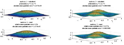
Figure 5.6. Examples of modes furnished by the Q2 family. For a color version of the figure, see www.iste.co.uk/souzadecursi/variational.zip
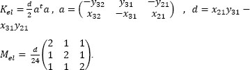
For T1 finite elements, rectangle Qij is split in two triangles by one of its diagonals. For instance, one triangle is limited by P1 = Pij, P2 = Pi+1,j, P3 = Pi+1,j+1, while another one is limited by P1 = Pij, P2 = Pi+1,j+1, P3. On each element, u is approximated by a polynomial function of degree 1 having as expression a0 + a1x1 + a2x2. Elementary mass and stiffness are usually evaluated as functions of P2 − P1 = (x21, y21), P3 − P1 = (x31, y31), P3 − P2 = (x32, y32);
Results furnished by T1 are shown in Figure 5.7.
When α is small, the geometry of the rectangle may be approximated by a line and we expect that the eigenvalues end modes converge to the corresponding ones for a biclamped bar:

Figure 5.7. Examples of modes furnished by the T1 family. For a color version of the figure, see www.iste.co.uk/souzadecursi/variational.zip
It is interesting to compare this value to the mean of a mode along the vertical axis:
As shown in Figure 5.8, umean and u1d are close.
![]()
5.4. Evolution partial differential equations
Let us consider the situation where
With
In this case, we have
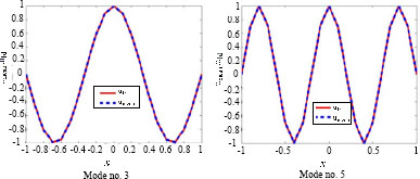
Figure 5.8. Comparison between the mean along the vertical axis and a one-dimensional mode (α = 0.1)
5.4.1. Linear equations
Let us assume that u → a(u, v) is linear. Using the approximation introduced in sections 4.4, 4.7 and 4.8:
and

where
In addition, we may approximate
In this case, we have
Thus,
These observations show that approximations of a linear differential equation using a total family or a Hilbert basis leads to the construction of:
- 1) a mass matrix M;
- 2) a stiffness matrix K;
- 3) a second member B, which may depends upon t;
- 4) an initial data U0.
For instance, these matrices may be generated by finite element methods (FEM) or the continuous families presented.
The resulting equations may be integrated by intrinsic solvers from Matlab® (ode45, ode23s, etc.). For instance, we may implement a subprogram evaluating M−1(B − KU). Denoting by invM the inverse M−1 of M and invMK the value of M−1K, we may use the code
function v = second_member(t,U,invM,invMK, B)
v = invM*B(t) - invMK*U;
end
Then, we call one of these solvers:
T = ...; % give the time interval (0,T)
solver = @solvername; % solvername: ode45,ode23s,etc.
invM = M  eye(size(M)); % evaluate inv(M)
invMK = M  K; % evaluate inv(M)*K
U0= M  Y; % vector of initial conditions
B = @program_name; % name of the subprogram evaluating
F.
secm = @(t,X) second_member(t,U,invM,invMK, B);
sol = solver(secm, [0,T], U0);
Returning structure sol contains:
- 1) sol.x : vector of time moments. The line tc = sol.x; copies the time moments in vector tc — the solution has been evaluated at tc(1), tc(2) — tc(end).
- 2) sol.y : array of values of U. Each colum of sol.y contains the solution for one time moment: column j (sol. y (: , j) ) contains the solution U at time tc(j). Each line contains the solution for a given degree of freedom (dof) and all the times: line i (sol. y (i , :) ) contains the evolution of Ui for all the values tc.
5.4.2. Nonlinear equations
Let us assume that u → a(u, v) is nonlinear. In this case,
and we have
where
Let us assume that proj(U,basis) furnishes Pu, while a (pu, basis) furnishes a vector v such that vi = a(PU, φi). In this case, the second member reads as
function v = second_member(t,U,invM,a, proj,basis,B)
pu = proj(U,basis);
aux = a(pu,basis) ;
v = invM*(B(t) -aux); % or M  (B(t) - aux) ;
end
Then, the differential equation may be solved by an intrinsic solver from Matlab®.
5.4.3. Motion equations
Let us consider the equations describing the motion of an undamped system:
The model must be completed by initial conditions:
The main assumption on this system concerns the existence of normal modes, i.e. the existence of vectors φi, i = 1, … , n (n = dimension of the square matrices M, K and of vector U), such that the matrix Φ = [ϕ1, …, ϕn] having as columns the vectors simultaneously diagonalizes the matrices M, K:
Where ![]() are diagonal matrices. The vectors are determined by setting
are diagonal matrices. The vectors are determined by setting
and solving
As an alternative, we may set
w is called a natural pulsation. Φ is the associated eigenvector, called normal mode.
We set
and the problem is rewritten as:
These equations correspond to evolution equations as treated in section 5.4.1. They may be integrated by intrinsic solvers from Matlab® (ode45, ode23s, etc.). The subprogram evaluating the right-hand side of this system reads as
function v = secm_matlab(t,X,invM, invMK,invMC,F)
n = length(X)/2;
v = zeros(size(X));
v(1: n) = X(n+1:2*n);
v(n+1:2*n) = invM*F(t) - invMK*X(1: n) -
invMC*X(n+1:2*n);
end
Subprogram F must be implemented independently and returns the force vector at time t.
Assuming that the values of U0, ![]() are defined in the Matlab vectors U0 and Up0, respectively, then Matlab® solver is called as follows:
are defined in the Matlab vectors U0 and Up0, respectively, then Matlab® solver is called as follows:
T = ...; % give the time interval (0,T)
solver = @solvername; % solvername: ode45,ode23s,etc.
invM = M  eye(size(M)); % evaluate inv(M)
invMK = M  K; % evaluate inv(M)*K
invMC = M  C; % evaluate inv(M)*C
X0 = [U0; Up0]; % vector of initial conditions
F = @program_name; % name of the subprogram evaluating
F.
secm = @(t,X) sec_matlab(t,X,invM, invMK,invMC, F);
sol = solver(secm, [0,T], X0);
5.4.3.1. Newmark integration of motion equations
One of the most popular numerical methods in dynamics is Newmark’s scheme:

Here, β, γ are strictly positive parameters to be defined by the user. For ![]() the method is unconditionally stable. Typical values are
the method is unconditionally stable. Typical values are ![]() For the system under consideration, we have:
For the system under consideration, we have:

or, equivalently,

Let us introduce a time discretization involving nt subintervals of time:
We denote
Thus

The first equation reads as
and determines Ui+1. Then, the second equation determines ![]() . A simple Matlab implementation is the following:
. A simple Matlab implementation is the following:
nt = …; % number of time intervals
dt = T/nt; % time step
F = @(t) program_name(t, …); % subprogram evaluating F.
betta = …; % value of beta.
gama = … ; % value of gama.
A = MM + betta*dt*dt*KK;
t = 0;
Ui = U0;
Vi = Up0;
Fi = F(t);
Ai = M  (Fi - K*Ui)
for npt = 1: nptmax
t = t + dt;
Fi1 = F(t);
    aux = M*Ui + dt*M*Vi + 0.5*dt*dt*((1-2*betta)*(Fi -
K*Ui) + 2*betta*Fi1);
    Ui1 = A aux;
    Ai1 = M  (Fi1 - K*Ui1);
Vi1 = Vi + dt*((1-gama)*Ai + gama*Ai1);
Ui = Ui1;
    Vi = Vi1;
    Ai = Ai1;
Fi = Fi1 ;
    end;
Newmark’s scheme also reads as the construction of a sequence of vectors given by
or

Since
we have
so that Newmark’s scheme reads as
with

The first equation furnishes a linear system for Uk+1. Once Uk+1 is determined, the second line furnishes ![]() . An alternative code is
. An alternative code is
nt = …; % number of time intervals
dt = T/nt; % time step
F = @program_name; % name of the subprogram evaluating
F.
betta = …; % value of beta.
gama = … ; % value of gama.
A1_11 =M + betta*dt*dt*K;
A1_21 = gama*dt*K;
A1_22 = M;
A2_11 = M - (0.5 - betta)*dt*dt*K;
A2_12 = dt*M;
A2_21 = -(1-gama)*dt*K;
A2_22 = M;
A3_11 = (0.5 - betta)*dt*dt;
A3_12 = betta*dt*dt ;
A3_21 = (1-gama)*dt;
A3_22 = (1-gama)*dt;
t = 0;
Uk = U0;
Upk = Up0;
Fk = F(t);
for npt = 1: nt
    t = t + dt;
Fk1 = F(t);
    B = A2_11*Uk + dt*M*Upk + A3_11*Fk + A3_12*Fk1;
    Uk1 = A1_11  B;
    B = - gama*dt*K*Uk1-(1-
gama)*dt*K*Uk+M*Upk+A3_21*Fk+A3_22*Fk1;
    Upk1 = M  B;
    Uk = Uk1;
    Upk = Upk1;
    Fk = Fk1;
end;
5.4.3.2. Fourier integration of motion equations
If
then
with

Here, ϕk are the eigenvectors and wk,nat are the natural pulsations associated to K. We have
The coefficients ![]() , UA, UB are determined by
, UA, UB are determined by
Let us introduce the matrix Φ = [ϕ1, … ,ϕn] having as columns the eigenvectors, Ωnat a diagonal matrix containing the natural frequencies in the diagonal, SINnat and COSnat, diagonal matrices containing the terms sin(wnat,kt) , cos(wnat,kt), respectively:
Then:
and
Analogously, let us consider Ω a diagonal matrix containing the frequencies wi in the diagonal, SIN and COS, diagonal matrices containing the terms sin(wit) , cos(wit), respectively:
Then

so that
Thus
which determines the coefficients A, B. A simple implementation of this method is the following one:
function [Ubar, U_A,U_B,a,b] =
solve_multichromatic(omega, M,K, Phi, om_nat, Fbar, F_A,
F_B, U0, V0)
U_A = cell(size(omega));
U_B = cell(size(omega));
Ubar = K Fbar;
for i = 1: length(omega)
om = omega(i);
    fA = F_A{i};
    fB = F_B{i};
    matsys = K - om^2*M;
uA = matsys  fA;
    uB = matsys  fB;
U_A{i} = uA;
    U_B{i} = uB;
end;
X_B = Ubar;
for i = 1:length(omega)
X_B = X_B + U_B{i};
end;
b = Phi  (U0 - X_B);
X_A = zeros(size(U_A{1}));
for i = 1:length(omega)
    X_A = X_A + omega(i)*U_A{i};
end;
gama = Phi  (V0 - X_A);
a = gama./om_nat;
return;
end
5.4.4. Motion of a bar
Let us consider a bar of length ℓ > 0, submitted to a distributed load f , clamped at origin and force fℓ extremity ℓ. The motion’s equations are
where:
- 1) E = Young’s modulus of the material;
- 2) S = surface of the right section;
- 3) ρ = volumetric density of the material.
FEM discretization starts by the generation of a set of vertices and elements, defined by a partition
Element number i is (xi, xi+1). When a uniform discretization is used, we have
In this case, we may generate the discretization and the elements by using the following matlab® code
ele = …; % give the value of ℓ
n = …; % give the number of elements
x = linspace(0, ele, n+1);
element = zeros(n,2);
for i = 1: n
    element(i,:) = [i i+1];
end;
The complete mass and stiffness cM, cK are generated by using integrals involving the shape functions on the elements, i.e. the elementary matrices me for mass and ke for stiffness. For instance, let us consider the classical bar element involving 2 degrees of freedom by element. In this case,
For instance, we may use the Matlab code
   elastmod = …; % give the value of Young's modulus
   surf = …; % give the value of the surface of the
right section
   rho = … ; % give the value of the volumetric density
of the material
   m_e = rho*surf*h*[2 1 ; 1 2]/6;
   k_e = elastmod*surf*[1 -1; -1 1]/h;
Matrices cM, cK are obtained by assembling the elementary matrices on the elements:
cM = zeros(n+1,n+1);
cK = zeros(n+1,n+1);
for i = 1:n
   ind = element(i,:);
   cM(ind, ind) = cM(ind, ind) + m_e;
   cK(ind, ind) = cK(ind, ind) + k_e;
end;
Boundary condition u(0, t) = 0 is taken into account by the elimination of the first line and column of cM, cK. For instance, we may use the code:
M = cM(2:n+1,2:n+1);
K = cK(2:n+1,2:n+1);
External forces are given by a time-dependent field f(x, t). Force vector is obtained by assembling the elementary forces: on element i, corresponding to nodes [i i+1] and degrees of freedom [i i+1], the forces are (fi, fi+1), fi = f(xi, t). Assembling is made by using the vector of nodal forces f = (f1, ... fn+1)t. Let us assume that the values of f, fℓ are furnished by subprograms f, f_ele, respectively. Then, an example of assembling is given by the subprogram
   function cF = assembly_force(f,f_ele,x,n,t, elastmod,
surf)
   cF = zeros(n+1,1);
   for i = 1: n
   dof = [i, i+1];
       f_el = [f(x(dof(1)),t), f(x(dof(2)),t)];
       cF(dof) = cF(dof) + mean(f_el)*[1; 1];
end;
cF(n+1) = CF(n+1) + f_ele(t)/(elastmod*surf);
return;
end
In this situation, assembling may be simplified:
At time t, this vector may be obtained by using the subprogram
   function cF = assembly_force(f,f_ele, x,n,t, cM,
elastmod, surf)
   f = zeros(n+1,1);
   for i = 1: n+1
   f(i) = f(x(i),t);
   end;
   cF = cM*f;
   cF(n+1) = cF(n+1) + f_ele(t)/(elastmod*surf); );
   return;
   end
The elimination of the first degree of freedom is performed as follows:
   function F = force(t,f,f_ele, x,n, cM, elastmod, surf)
   cF = assembly_force(f,f_ele, x,n,t, cM, elastmod,
surf);
   F = cF(2:end);
   return;
   end
Initial conditions are discretized as follows: assume that the values of u0(x), u0(x) are furnished by subprograms u_0, up_0, respectively. Then, we may use the code
cU0 = zeros(n+1,1);
cUp0 = zeros(n+1,1);
for i = 1: n+1
    cU0(i) = u_0(x(i));
cUp0(i) = up_0(x(i));
end;
U0 = cU0(2:n+1);
Up0 = cUp0(2:n+1);
EXAMPLE 5.7.— A uniform monochromatic force
Let us consider the bar submitted to the oscillating forces
For
omega = 1;
pA = 1;
pB = 2;
f = @(x,t) pA*sin(omega*t) + pB*cos(omega*t);
f_ele = @(t) 0;
we have the results below for the motion of the last node.

EXAMPLE 5.8.— A uniform multichromatic force
Let us consider the bar submitted to the oscillating forces
For
omega = [ 1 2 3 4];
pA = [ 4 3 2 1];
pB = [ 1 2 3 4];
pbar = 0;
f = @(x,t) somme_trigo(x,t, pbar, pA, pB, omega);
f_ele = @(t) 0;
we have the results below for the motion of the last node.

5.4.5. Motion of a beam under flexion
Let us consider a beam of length ℓ > 0, submitted to pure flexion under a distributed load f, clamped at origin and force fℓ, extremity ℓ. The motion’s equations are
where:
- 1) E = Young’s modulus of the material;
- 2) S = surface of the right section;
- 3) I = inertia moment of the cross section;
- 4) ρ = volumetric density of the material.
FEM discretization is analogous to the preceding one. For instance, let us consider the classical beam element involving 4 degrees of freedom by element. In this case,

For instance, we may use the Matlab code
   elastmod = ...; % give the value of Young's modulus
   surf = ...; % give the value of the surface of the
right section
   rho = ... ; % give the value of the volumetric density
of the material
   inertia = ... ; % give the value of the inertia of the
right section
   m_el = rho*surf*h*[
   156 22*h 54 -13*h;
              22*h 4*h^2 13*h -3*h^2;
              54 13*h 156 -22*h;
              -13*h -3*h^2 -22*h 4*h^2
          ]/420;
   k_el = elastmod*inertia*[
          12 6*h -12 6*h;
          6*h 4*h^2 -6*h 2*h^2;
          -12 -6*h 12 -6*h;
          6*h 2*h^2 -6*h 4*h^2
   ]/h^3;
Analogously to the preceding situation, matrices cM, cK are obtained by assembling the elementary matrices on the elements:
ndof = 2*(n+1);
cM = zeros(ndof,ndof);
cK = zeros(ndof,ndof);
for i = 1: n
ind = (2*i-1:2*i+2);
    cM(ind,ind) = cM(ind,ind) + m_el;
    cK(ind,ind) = cK(ind,ind) + k_el;
end;
Boundary conditions u(0, t) = u′(0, t) = 0 are taken into account by the elimination of the two first lines and columns of cM, cK. For instance, we may use the code:
M = cM(3:ndof,3:ndof);
K = cK(3:ndof,3:ndof);
External forces are given by a time-dependent field f(x, t). The force vector is obtained by assembling the elementary forces: on element i, corresponding to nodes [i i+1] and degrees of freedom [2*i−1 2*i 2*i+1 2*i+2], the forces are (fi, fi+1), fi = f(xi, t). An example of assembling is given by the subprogram
   function cF = assembly_force(f,f_ele,x,n,t, elastmod,
inertia)
   cF = zeros(2*n+2,1);
   for i = 1: n
       dof = (2*i-1:2*i+2);
       f_el = [f(x(i),t); f(x(i+1),t)];
       cF(dof) = cF(dof) + mean(f_el)*h*[1; h/6; 1; -
h/6]/2;
   end;
   cF(2*n+1) = CF(2*n+1) + f_ele(t)/(elastmod*inertia);
   return;
   end
The elimination of the two first degrees of freedom is performed as follows:
   function F = force(t,f,f_ele, x,n, cM, elastmod,
inertia)
   cF = assembly_force(f,f_ele, x,n,t, cM, elastmod,
inertia);
   F = cF(3:end);
   return;
   end
Initial conditions are discretized analogously to the case of a bar.
EXAMPLE 5.9.— A uniform monochromatic force
Let us consider the beam submitted to the oscillating forces
For
omega = 1;
pA = 1;
pB = 2;
f = @(x,t) pA*sin(omega*t) + pB*cos(omega*t);
f_ele = @(t) 0;
we have the results below for the motion of the last node.

EXAMPLE 5.10.— A uniform multichromatic force
Let us consider the beam submitted to the oscillating forces
For
omega = [ 1 2 3 4];
pA = [ 4 3 2 1];
pB = [ 1 2 3 4];
pbar = 0;
f = @(x,t) somme_trigo(x,t, pbar, pA, pB, omega);
f_ele = @(t) 0;
we have the results below for the motion of the last node.

5.5. Exercises
EXERCISE 5.1.— Let V = H1(Ω)
- 1) Show that there exists M
 such that: ∀v V: |ℓ(v)|≤ M || ||1.
 - 2) Conclude that there exists one and only one u V such that (u, v)0 = ℓ(v),∀v V.
- 3) Show that u(x) = 1 on Ω.
EXERCISE 5.2.— Let Ω = (0,1), a ![]() Ω, P
Ω, P ![]() R, c
R, c ![]() L2(Ω). Let F(v) = Pv(a) + (c, v)0 ; (u, v)0 = ∫Ω uv.
L2(Ω). Let F(v) = Pv(a) + (c, v)0 ; (u, v)0 = ∫Ω uv.
- 1) Show that

- 2) Let V = {v H1(Ω)|v(0) = v′(0) = 0} and the scalar product

- 3) Let (v) = Pv(a) + (c, v)0. Use exercise 4.10 to show that there exists one and only one u V such that ∀ v V : (u, v)v + C(v) = 0
- 4) Assume that u
 L2 (Ω).
- a) Show that

- b) Conclude that Pφ(a) + (u + c, φ)0 = 0, ∀φ D(Ω).
- c) Show that P = 0 and u + c = 0 on Ω.
- d) Show that u(0) = u′(0) = u″(1) = u
 (1) = 0
- a) Show that
- 5) Assume that u L2(0, a), u L2(a, 1), [u(a)] = u(a+) − u(a−) .
- a) Show that, ∀ v V:
- b) Conclude that


- c) Show that P + [u(a)] = 0 and u + c = 0 on Ω.
- d) Show that u(0) = u′(0) = u″(l) = u(l) = 0.
- a) Show that, ∀ v
- 6) Let J:V → R be given by
 . Let u* =
  .
.
- 1) Let g(λ) = J(u* + λv), λ Verify that, ∀v ∈ V, the minimum of g is attained at λ = 0.
- 2) Use that g′(0) = 0 in order to conclude that (u*, v)v + C(v) = 0, ∀v ∈ V
- 3) Conclude that u* = u
![]()
EXERCISE 5.3.— Let Ω ⊂ R2 be a regular bounded domain,
The scalar product on V is defined as
Let us introduce
- 1) Show that there exists a constant C such that ∀v ∈ V: ||v||2 ≤ C||v||v.
- 2) Verify that S is a vector subspace from V.
- 3) We aim to show that S is closed.
- 1) Verify that v ∈ S ⇔ (v, ∇φ)0,2 = 0, ∀φ ∈ D(Ω).
- 2) Let {un: n ∈
 }n ⊂ S satisfy un → u strongly in (V, ||v||v). Verify that ||un − u||2 ≤ C||un − u||v. Show that (un − u, ∇φ)0 → 0.
 - 3) Conclude that S is closed.
- 4) Let η ∈ V satisfy (η, v)0 = 0, ∀v ∈ S. We aim to show that η = ∇ψ: it suffices to show that rot (v) = 0.
- 1) Verify that ∀φ ∈ D(Ω) : v = (∂2φ, −∂1φ) ∈ S.
- 2) Show that (∂1η2 − ∂2η1, φ)0,2 = 0,∀φ ∈ D(Ω).
- 3) Conclude.
- 5) Let b(u,v,w) = ((u.∇)(v), w)0.
- a) Show that

- b) Verify that

- c) Show that

- d) Show that

- a) Show that
- 6) Let

- a) Show that there exists a constant K ∈ such that ∀v ∈ V :|F(v)|≤ K ||v||V.
- b) Verify that F ∈ V′.
- a) Show that there exists a constant K ∈
- 7) Let a(u, v) = (u, v)V + b(u, u, v).
- a) Show that

- b) Verify that

- a) Show that
- 8) Let u be the solution of

We aim to show that u verifies the Navier-Stokes’ equations
a) Show that ![]() .
.
b) Verify that
4) Show that there exists p: Ω → R such that Δu − (u. Δ)(u) + f = Δp
5) Conclude.
EXERCISE 5.4.— Let Ω ⊂ R2 be a regular bounded domain,
with the scalar product
We assume that λ > 0, λ + 2μ ≥ 0.
- 1) Verify that

- 2) Let

Show that .
. - 3) Conclude that A = 0 and div(u) = 0 ⇔ ∇u = 0.
- 4) Show that

- 5) Conclude that (•,•)V is a scalar product on V .
- 6) Let F ∈ V′. Show that there exists a unique u ∈ V such that

- 7) Show that

- 8) Show that

- 9) Show that

- 10) Let
 . Show that
- 11) Conclude that

