
7
Functionals and Calculus of Variations
For people interested in ancient myths, calculus of variations may be dated from the creation of Carthage by Elissa (also called Dido). This mythical phenycian queen which “bought all the land she could enclosed with a bull’s hide” (“mercatique solum, facti de nomine Byrsam, taurine quantum possent circumdare tergo” [VIR 19]), delimited a circle using a string made of tires cut in a bull’s hide. In fact, philosophers have long considered the connections between area and perimeter and looked for the maximal area for a given length (namely Zenodorus the Greek and Pappus of Alexandria) and Hero of Alexandria formulated a principle of economy, which corresponds to a variational principle.
Other people date calculus of variations from the famous problem stated by Johann Bernouilli about the brachistochrone ([BER 96], even if the same problem had already been proposed by Galilei Galileo precedently [GAL 38, ERL 88] – in addition, Fermat and Huyghens previously formulated physical principles leading to problems of Calculus of variations.
The basic problem of calculus of variations consists of determining a field that realizes the minimum or the maximum of a real quantity associated with it, such as, for instance, the energy, the area, the length, a characteristic time, etc. In the case of a real function f: ![]() →
→ ![]() , such a point x verifies f'(x) = 0, meaning that the tangent to the curve (x, f(x)) is a horizontal straight line. The extension of such a result, to the situation where f becomes energy and x becomes a field, requests the definition of derivatives for functions of functions.
, such a point x verifies f'(x) = 0, meaning that the tangent to the curve (x, f(x)) is a horizontal straight line. The extension of such a result, to the situation where f becomes energy and x becomes a field, requests the definition of derivatives for functions of functions.
A first analysis was made by Vito Volterra, which introduced the first definition of functional derivatives [VOL 87]. Jacques Hadamard remarked the works of Volterra and met him at conferences such as the International Congress of Mathematics, in 1897 in Zurich (then 1900 in Paris and 1904 in Heildelberg). Hadamard was interested in the ideas of Volterra on functional calculus and introduced the terminology functional in order to describe the “ functions of lines” of Volterra [HAD 02, HAD 03a, HAD 10]. Hadamard had a student – Maurice Fréchet – who rapidly developed a new theory about differentials of functions of functions [FRE 04, FRE 11a, FRE 11b, FRE 12, FRE 14]. Fréchet also published the notes of a course by Hadamard about this subject [HAD 10].
The works of Fréchet did not end the discussion about differentials of functions. A young mathematician, René Eugène Gâteaux, proposed a new point of view, based on the extension of the notion of directional derivative. In fact, René Gâteaux was interested in extensions of Riezs’s theorems to nonlinear situations, i.e. in the representation of nonlinear functional [GAT 13a, GAT 13b, GAT 14a, GAT 14b]. A simple approach in order to generate such a representation consists of the use of expansions analogous to the Taylor series. These questions were investigated, namely by Volterra, Hadamard and Fréchet, and led to the theory of functional derivatives. Some of Gâteaux’s results [GAT 19a, GAT 19b, GAT 22] were published after his death in October 1914, during a battle in World War I, but his approach has been shown to be very convenient in practical situations, which explains the popularity of Gâteaux derivatives.
7.1. Differentials
Let us consider a regular function f: ![]() →
→ ![]() . In fact, the value df/dt does not represent the variations of f, but gives the slope of the tangent line to the graphics of the function at the point (x, f(x)).
. In fact, the value df/dt does not represent the variations of f, but gives the slope of the tangent line to the graphics of the function at the point (x, f(x)).
The variations of f are represented by its differential df, which is a mathematical object of a different kind: df is a linear function that locally approximates f (x + δx) – f (x). In other terms, we have df(x) = T, where T is a linear junction such that f (x + δx) – f (x) ≈ T (δx). So,
df (x)(δx) is the first-order approximation of f (x + δx) – f (x):
These elements are illustrated in Figure 7.1.

Figure 7.1. Differential of a functional. For a color version of the figure, see www.iste.co.uk/souzadecursi/variational.zip
7.2. Gâteaux derivatives of functionals
An interesting property of df is the following:
The value df (x)(δx) is called the Gâteaux derivative of f at the point x in the direction δx. The linear application δx → df (x)(δx) is the Gâteaux differential of f at x. These notions extend to energies defined for physical fields. Let us recall a fundamental definition:
DEFINITION 7.1.– Let V be a vector space. A functional is an application J: V → ![]() .
.
![]()
Thus, a functional is simply a function defined on V, taking its values on the real line ![]() . Functionals are used in order to represent energies, distances between desired states and effective ones, or quantities defined in order to give a numerical measurement of some qualitative criteria. Namely, energies, variations of energy and virtual works are represented by functional. In section 3.9.1, we have considered a particular class formed by linear functionals, i.e. functionals ℓ:V→
. Functionals are used in order to represent energies, distances between desired states and effective ones, or quantities defined in order to give a numerical measurement of some qualitative criteria. Namely, energies, variations of energy and virtual works are represented by functional. In section 3.9.1, we have considered a particular class formed by linear functionals, i.e. functionals ℓ:V→![]() verifying ℓ(u + λv) = ℓ(u) + ℓ(v)∀ u, v ∈ V, λ ∈
verifying ℓ(u + λv) = ℓ(u) + ℓ(v)∀ u, v ∈ V, λ ∈ ![]() . For instance, virtual works are linear functionals in the space V formed by the virtual motions.
. For instance, virtual works are linear functionals in the space V formed by the virtual motions.
DEFINITION 7.2.– Let V be a vector space and J:V → ![]() be a functional. The Gâteaux derivative of J at the point u ∈ Vin the direction δu is:
be a functional. The Gâteaux derivative of J at the point u ∈ Vin the direction δu is:
![]()
The linear functional V ∋ δu → dJ(u)(δu) ∈ ![]() is the Gâteaux differential of J at the point u.
is the Gâteaux differential of J at the point u.
![]()
We have our first result:
THEOREM 7.1.– Let V be a vector space and ℓ: V → ![]() be a linear functional. Then:
be a linear functional. Then:
![]()
PROOF.– We have ℓ(u + λδu) = ℓ (u) + λℓ (δu) so that:
and we have ![]()
![]()
Let us recall that u ∈ V achieves the minimum of J on C ⊂ V – or that u is the optimal point of J on C – if and only if u ∈ C and J (u) ≤ J(v), ∀ v ∈ V. In this case, we write:
The second result is the following:
THEOREM 7.2.– Let V be a vector space and J: V → ![]() be a Gâteaux-differentiable functional. Let,
be a Gâteaux-differentiable functional. Let,
![]()
PROOF.– Let δu ∈ V and λ > 0. Then, we have u + λδu ∈ V and u –
λδu ∈ V,so that:
Since λ > 0,

Thus, by taking the limit for λ → 0 +:
Since δu → DJ(u)(δu) is linear, we have DJ(u)(–δu) = –DJ(u)(δu), so that DJ(u)(δu) ≥ 0 and – DJ(u)(δu) ≥ 0, what shows that DJ (u) (δu) = 0.
![]()
The third result is the following:
THEOREM 7.3.– Let C ⊂ 7 be a non-empty convex subset (see section 3.7.2) and
Then, DJ(u)(δu) ≥ 0, ∀ δu such that u + δu ∈ C or, equivalently,
![]()
PROOF.– Let δu ∈ V verify u + δu ∈ C and λ ∈ (0,1). Then, convexity of C implies that u + λδu = (1 – λ) u + λ (u + δu) ∈ C, so that:
Thus, by taking the limit for λ → 0 +, we obtain DJ(u)(δu) ≥ 0. Finally, we observe that v ∈ C ⇒ δu = v – u verifies v = u + δu ∈ C, so that we have the result.
![]()
7.3. Convex functionals
DEFINITION 7.3.– Let V be a vector space and J: V → ![]() be a functional. We say that J is convex if and only if
be a functional. We say that J is convex if and only if
![]()
Convexity of a functional may be interpreted as shown in Figure 7.2: let
The curve formed by the points (θ, f(θ)) remains inferior to the segment of line connecting the points (0, J (v)) and (1, J(u)).

Figure 7.2. A convex functional
We have:
THEOREM 7.4.– Let V be a vector space and J: V → ![]() be a Gâteaux-differentiable functional. Assume that J is convex. Then:
be a Gâteaux-differentiable functional. Assume that J is convex. Then:
![]()
PROOF.– Let u, v ∈ V and θ ∈ (0,1). Then,
Since
so that:
Taking the limit for θ → 0 +: DJ (u)(v–u) ≤ J(v) – J(u)
![]()
THEOREM 7.5 – Let V be a vector space and J: V → ![]() be a Gâteaux-differentiable functional. Assume that J is convex and u ∈ V verifies
be a Gâteaux-differentiable functional. Assume that J is convex and u ∈ V verifies
![]()
PROOF.– Let v ∈ V. From theorem 7.4: J(v) – J(u) ≥ DJ(u)(v – u) = 0. Thus, J(v) ≥ J(u). Since v is arbitrary, we have u = arg min {J(v): v ∈ v}
![]()
THEOREM 7.6 – Let V be a vector space and J: V → ![]() be a Gâteaux-differentiable convex functional. Then
be a Gâteaux-differentiable convex functional. Then
![]()
PROOF. – We have:

Adding these two inequalities,
so that:
THEOREM 7.7 – Let C ⊂ V be a not empty convex set and J: V → ![]() be a Gâteaux-differentiable functional. Assume that J is convex and u ∈ C verifies DJ(u)(δu) ≥ 0, ∀δu such that u + δu ∈ C (or, equivalently, DJ(u)(v – u) ≥ 0, ∀v ∈ C). Then u = arg min {J(v): v ∈ V}.
be a Gâteaux-differentiable functional. Assume that J is convex and u ∈ C verifies DJ(u)(δu) ≥ 0, ∀δu such that u + δu ∈ C (or, equivalently, DJ(u)(v – u) ≥ 0, ∀v ∈ C). Then u = arg min {J(v): v ∈ V}.
PROOF. – We have:
so that J (v) ≥ J(u), ∀u ∈ C and we obtain the result.
7.4. Standard methods for the determination of Gâteaux derivatives
7.4.1. Methods for practical calculation
The practical evaluation of Gâteaux differentials is performed by using one of the following methods:
1) Derivatives of a real function: let us consider a point u ∈ V, a virtual motion δu ∈ V. We set, for λ ∈ ![]() , f(λ) = J(u + λδu). Then
, f(λ) = J(u + λδu). Then
2) Local expansions limited to first-order: let us consider a point u ∈ V, a virtual motion δu ∈ V. We have for λ ∈ ![]() , f(λ) = J(u + λδu). Then
, f(λ) = J(u + λδu). Then
However, we may take f(λ) = J(u + λδu) and approximate
Thus, we may consider the expansion:
and we have DJ(u)(δu) = B.
EXAMPLE 7.1. – For instance, let us consider the simple system formed by a mass m and a spring having rigidity k and natural length x0, under the action of a force f.

The position of the mass at time t is x(t) and its initial position is x(0) = x0. The displacement of the mass is u(t) = x(t) – x0. The kinetic energy of the mass is:
We have:
where,
Thus,
However,
and we have DK(u)(δu) = B again.
However, the elastic energy of the spring is:
In this case,
where:
Thus,
However,
and we have yet DW(u)(δu) = B.
Finally, the potential due to the force f is;
This expression corresponds to a linear functional. Thus,
![]()
7.4.2. Gâteaux derivatives and equations of the motion of a system
In Lagrange’s formalism, the motion of a system is described by using Gâteaux differentials: let q = (qt, …, qn) be the degrees of freedom of the system. Assume that the Kinetic energy is K(q, ![]() ), while the potential energy isV(q). The Lagrangian of the system is L = K–V and the action of the system is:
), while the potential energy isV(q). The Lagrangian of the system is L = K–V and the action of the system is:
Let us consider δq such that δq(0) = δq(T) = 0. Then, the motion is described by:
This variational equation corresponds to the following system of differential equations:
These last equations are known as Euler–Lagrange’s equations associated with the Lagrangian L.
EXAMPLE 7.2. – As an example, let us consider the system shown in Figure 7.4. In this case, n = 1 and q1 = u. We have;
so that:
and
i.e.
Integrating by parts, we obtain:
which implies that:
Thus, mü = f – ku on (0, T).We observe that:
So, Euler–Lagrange’s equations read as:
![]()
EXAMPLE 7.3. – Let us consider again the situation shown in section 6.1. Let us introduce a slight modification in the standard Newton’s law: the original one states that force = change in motion = change in [mass x velocity]. From the variational standpoint, only changes in energy have to be considered and Newton’s law becomes work for a variation δu on a time interval (t1, t2) = change in energy for δu on (t1, t2) = change in [mass x velocity2/2] for δu on (t1, t2). Thus, we consider:
We look for a linear approximation T such that:
As previously observed, we may determine the approximation by evaluating the Gâteaux differential of K:
As previously, indicated, we may consider Ω = (t1, t2) and the set of test functions,
D(Ω)={φ:Ω→R : ∃ ω⊂Ω, ω closed and bounded, φ(x)=0 if x∉ω}.
All the elements of D(Ω) vanish at the ends of the interval: φ(t1) = φ(t2) = 0, ∀φ ∈ D(Ω). We evaluate T (φ) for φ ∈ D(Ω): whenever,
f is the force generating the change in the kinetic energy of the mass. As previously established, we have:
If t1 <t2,<0 we have:
If 0 <t1 <t2, we have:

and we have f = 0 again. If t1 < 0 < t2, we have:
and T =mv0δ0, where δ0 is the Dirac’s mass supported by the origin x = 0. As previously observed, δ0 is not a usual function. It is a distribution; i.e., a linear functional T defined on ![]() (Ω).
(Ω).
![]()
7.4.3. Gâteaux derivatives of Lagrangians
A particular situation often found concerns functional J(u) defined by integrals involving u and its derivatives. This situation corresponds to Lagrangians.
1) If
Then
2) More generally, let ![]() and
and ![]()
Then
3) Analogously, let
If
Then
7.4.4. Gâteaux derivatives of fields
The notion of Gâteaux derivative extends straightly to the situation where a field X is a function of u: w = W(u). In this case, we may consider
In practice, w is often defined by an equation involving w, u and their derivatives. For instance, let us assume that:
Let us introduce
and assume that:
Since, for φ ![]()
![]() (Ω),
(Ω),
we have:

Let us assume that F is regular enough in order to have an expansion:
Then, the equality:
yields that
and we have:
Thus, δw is the solution of a differential equation. Under similar assumptions, the case where,

leads to the differential equation:
7.5. Numerical evaluation and use of Gâteaux differentials
Gâteaux differentials may be used in conjunction with Hilbertian basis in order to obtain numerical values, to implement descent methods, or to determine optimal points associated with Lagrangians. The basic use consists of either determining a derivative or solving an equation concerning the Gâteaux differential. In the following, {φn}n ∈ ![]() is a total family (such as, for instance, a Finite Element one) or a Hilbertian basis (such as, for instance, Legendre Polynomials).
is a total family (such as, for instance, a Finite Element one) or a Hilbertian basis (such as, for instance, Legendre Polynomials).
7.5.1. Numerical evaluation of a functional
As observed above, the numerical evaluation of a functional may be performed by using a total family or a Hilbert basis. For instance, we may use the families defined in section 2.2.6.
A situation often found in practice consists of functional defined by Lagrangian densities:
fℓ is the Lagrangian density. If u and u′ are furnished as subprograms, we may evaluate J(u) by using numerical integration, as in section 1.5. If they are given as tables of data, we may use the methods presented in section 1.3. As an example, let us consider the situation where,
Let a = 0, b = 2π, u1(t) = 2 cos(t), u2(t) = 2 sin(t). The exact value is J(u) = 4π. The code
f_ell = @(t,u,du) sqrt(du(1)^2 + du(2)^2);
a = 0;
b = 2*pi;
%
u = @(t) 2*[cos(t), sin(t)];
du = @(t) 2*[-sin(t), cos(t)];
%
xlim.lower.x = a;
xlim.upper.x = b;
xlim.dim = 1;
g = @(t) f_ell(t, u(t), du(t));
sp = subprogram_integration(g,xlim);
v1 = sp.result ;
produces v1 = 12.5664≈4π. If the data is furnished as a table of values, we may use the class Riemann:
ns = 500;
h = (b-a)/ns;
x = a:h:b;
F = spam.points('vector',g,x);
p.x = x;
p.dim = 1;
p.measure = b-a;
data.points = p;
data.values = F;
v2 = riemann.trpzd(data);
This code produces the result v2 = 12.5664≈4π.
Assuming that an approximation ![]() is given, we may approximate,
is given, we may approximate,
For instance, let us consider the approximation of vector u(t) = 2(cos(t), sin(t)) in a polynomial basis φi(t) = ti–1 given by its orthogonal projection Pu on this basis. For n = 10, we obtain v1 = 12.5663 ≈ 4π.
Notice that J(Pu) is a function of the vector of coefficients U = (u1, …, un).
7.5.2. Determination of a Gâteaux derivative
Assume that a point ![]() , is given. The Gâteaux derivative J′(u) ∈ V is approximated as follows:
, is given. The Gâteaux derivative J′(u) ∈ V is approximated as follows: ![]()
![]() and we have:
and we have:
Thus,
which leads to a linear system A. P = B where
Once this system is solved for the coefficients P, the approximated value of ![]() is determined.
is determined.
As an example, let us consider Ω = (a, b) and the Lagrangian density:
We have:
Functional j has a meaning in Sobolev space H1(Ω), i.e. for the scalar product:
This scalar product may be defined as follows:
xlim.lower.x = a;
xlim.upper.x = b;
xlim.dim = 1;
sp0 = @(u,v) subprogram_integration(@(t)
u(t)*v(t),xlim).result;
sp1 = @(u,v,du,dv) sp0(u,v) + sp0(du,dv);
We have Dj(u)(v) = (u, v)1, so that, when using this scalar product, p = u. Functional J has also a meaning in Sobolev space V = {v ∈ H1(Ω): v(a) = 0} with the scalar product:
This scalar product may be defined by the code:
sp10 = @(u,v,du,dv) sp0(du,dv);
In this case, the equality
is integrated by parts, which leads to:
Thus,
Let us consider u(t) = sin (t), a = 0, b = 2π. For scalar product (![]() ,
, ![]() )1, we have p(t) = sin (t), while scalar product (
)1, we have p(t) = sin (t), while scalar product (![]() ,
, ![]() )1,0 corresponds to p(t) = 2 sin(t) – t. When using (
)1,0 corresponds to p(t) = 2 sin(t) – t. When using (![]() ,
, ![]() )1, the family is φi(t) = ti–1 with n = 10, which may be created as follows:
)1, the family is φi(t) = ti–1 with n = 10, which may be created as follows:
n = 10;
phi = polynomial_basis(0,0,1,n-1);
bp = basis(phi);
The coefficients may be determined by using
A = zeros(n,n);
B = zeros(n,1);
for i = 1: n
    phi1 = @(t) bp.phi.value(i,t);
    dphi1 = @(t) bp.phi.d1(i,t);
    A(i,i) = sp1(phi1,phi1,dphi1,dphi1);
    fff = @(t) df_ell(t,u(t),du(t),phi1(t),dphi1(t)) ;
    aux = subprogram_integration(fff,xlim);
    B(i) = aux.result;
    for j = i+1: n
    phi2 = @(t) bp.phi.value(j,t);
    dphi2 = @(t) bp.phi.d1(j,t);
        aux = sp1(phi1,phi2,dphi1,dphi2);
        A(i,j) = aux;
        A(j,i) = aux;
    end;
end;
U = A  B;
Then, p = bp.projection(U,tc) produces a table of values p(j) = p(tc(j)), for a given table of time moments tc.
For the scalar product (![]() ,
, ![]() )1,0, the family is φi(t) = ti with n = 10. The results are exhibited in the Figure 7.4.
)1,0, the family is φi(t) = ti with n = 10. The results are exhibited in the Figure 7.4.

Figure 7.4. Determination of a Gâteaux derivative for two different scalar products
It must be noticed that an attempt to use the scalar product (![]() ,
, ![]() )0 fails, except in particular situations: indeed, the equation
)0 fails, except in particular situations: indeed, the equation
leads to:
This variational equation does not have any solution, except in the case where u'(b) = u'(a) = 0. In this case, the solution is p = u – u". For instance, when considering u(t) = sin (t), a = 0, b = 2π, these conditions are not satisfied, since u'(b) = u'(a) = 1 and p does not exist.
7.5.3. Determination of the derivatives with respect to the Hilbertian coefficients
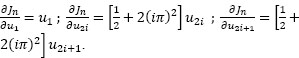
In some situations, we are interested in the evaluation of ∂j/∂ui, where ![]() . In this case, we consider U = (u1, … , un) and the function Jn :
. In this case, we consider U = (u1, … , un) and the function Jn : ![]() n →
n → ![]() defined by:
defined by:
The aim is to determine ∂Jn/∂ui. By considering the function:
it may be easily verified that:
As an example, let us consider Ω = (0,1) and the Lagrangian density
for which
Let us consider the trigonometric family φ1(t) = 1, φ2i(t) = cos(2iπt) φ2i+1 (t) = sin(2iπt). This family is orthogonal and ![]() ,
, ![]() , so that
, so that
And we have:
We may obtain a numerical evaluation by using the class


Then, we generate the family by:
n = 3;
phi = periodic_trigonometrical_basis(0,0,1,n);
bp = basis(phi);
We generate the gradient of Jn at the point U = (u1, … , un) as follows:
gradjn = zeros(size(U));
for i = 1: bp.nel
    phi1 = @(t) bp.phi.value(i,t);
dphi1 = @(t) bp.phi.d1(i,t);
u = @(t) bp.projection(U,t);
    du = @(t) bp.derive(U,t);
    fff = @(t)
df_ell(t,u(t),du(t),phi1(t),dphi1(t)) ;
aux = subprogram_integration(fff,xlim);
    gradjn(i) = aux.result;
   end;
For n = 3 and U=ones(2*n+1,1), we have:
gradjn=[1.0000 20.2392 20.2392 79.4568 79.4568 178.1529 178.1529],
which corresponds to the exact values.
7.5.4. Solving an equation involving the Gâteaux differential
Let F: V → ![]() be a linear functional. The numerical determination of u such that:
be a linear functional. The numerical determination of u such that:
is performed by setting ![]() and considering the set of n equations for the n unknowns U = (u1, … , un):
and considering the set of n equations for the n unknowns U = (u1, … , un):
This set of equations corresponds to:
It must be solved for the unknown U by appropriate numerical methods, such as, for instance, Newton-Raphson, fixed point, relaxation, least squares etc. Once the solution is determined, the approximation ![]() may be calculated.
may be calculated.
As an example, let us consider Ω = (0,1), V = H1(Ω) and the Lagrangian density:
for which:
Let us consider F(v) = (f, v)0. Then, the equality DJ(u)(δu) = F(δu) reads as:
Thus,
For instance, if f(t) = (1 + π2)sin (πt), then u(t) = sin (πt). Let us consider the trigonometric family φ1(t) = 1, φ2i(t) = cos(2iπt), φ2i+1(t) = sin (2iπt). As previously remarked, this family is orthogonal and verifies,
Moreover,
which determines the coefficients. Numerically, we may evaluate the vector E(U) = (E1(U), … , En(U) by the subprogram.
function eq = eqsdergat(U,basis,df_ell,xlim,f)
eq = zeros(basis.nel,1);
for i = 1: basis.nel
    phi1 = @(t) basis.phi.value(i,t);
    dphi1 = @(t) basis.phi.d1(i,t);
    u = @(t) basis.projection(U,t);
    du = @(t) basis.derive(U,t);
    fff = @(t) df_ell(t,u(t),du(t),phi1(t),dphi1(t)) ;
    aux1 = subprogram_integration(fff,xlim);
    fff = @(t) f(t)*phi1(t) ;
    aux2 = subprogram_integration(fff,xlim);
    eq(i) = aux1.result - aux2.result;
end;
end
Then, we generate a function of U as follows:
f = @(t) (1+pi^2)*sin(pi*t);
eq = @(U) eqsdergat(U,bp,df_ell,xlim,f);
Then we may solve the system eq = 0 by an adequated method. For instance, we may minimize fobj = @(U) norm(eq(U)). The point
U = [6.9198 -0.1140 0 -0.0058 0 -0.0011 0]
corresponds to fobj(U) ≈ 3.1 × 10⁻¹⁵. It is very close to the exact value.
7.5.5. Determining an optimal point
The numerical determination of u such that:
may be performed by different approaches:
1) Optimization approach: consider the function
previously introduced and determined a numerical solution of the problem
Analogously to the preceding situations, we have ![]() .
.
2) Optimization approach involving Gâteaux derivative: from the numerical standpoint, an alternative consists of using a descent method where the gradients are evaluated by using the Gâteaux derivative. For instance, the gradient descent with a fixed step reads as:
More generally, a descent direction d(k) must be determined by using information furnished by the preceding iterations and J′(u(k)). Classical methods for the determination of d(k) are gradient, Fletcher–Reeves, DFP, BFGS, etc. Once d(k) is known, we must determine a step µ(k) ≥ 0 in order to generate a new point by
Usual methods for the determination of µ(k) may be found in the literature. For instance, optimal step, fixed step, Armijo’s, Wolfe’s, and Goldstein’s approaches may be used. In practice, this approach may request finite-dimensional approximations ![]()
3) Equation approach: solve the equation DJ(u) = 0, i.e. the n equations for the n unknowns U = (u1, … , un):
Then, approach ![]() . Notice that the equation approach is not generally equivalent to the optimization one: convexity assumptions are requested for the equivalence.
. Notice that the equation approach is not generally equivalent to the optimization one: convexity assumptions are requested for the equivalence.
7.6. Minimum of the energy
In physics, one of the most useful principles is the principle of the minimum of the energy, which may be seen as a consequence of the second principle of thermodynamics – as formulated by Ludwig Boltzmann, the entropy can never decrease for an adiabatic system: thus, if S is the entropy such a system, we have dS ≥ 0 (otherwise, we have the Clausius-Durhem's inequality). As a consequence, for any isolated system, equilibrium corresponds to both a maximum of the entropy and a minimum of the energy – we say that these two principles are dual: there is a duality between maximum of entropy and minimum of energy. In mathematical terms, we must consider:
- 1) the space of the parameters: a Hilbert space V ;
- 2) the energy: a functional J: V →
 .
.
Then, the principle of the minimum of the energy states that equilibrium parameters u correspond to (recall that DJ(u) is the Gâteaux differential of J at the point u).
EXAMPLE 7.4. – Let us consider a system formed by a mass m, a spring having rigidity k under the action of the gravity f = mg (Figure 7.5)

Figure 7.5. Situation of example 7.4
Let us denote by u the displacement of the mass. Here, u ∈ V = ![]() . The energy of the system is:
. The energy of the system is:

Thus,
and the equilibrium corresponds to ku = mg = f.
![]()
If the system is submitted to some restrictions, the space of the parameters is not the whole space V : we must consider the admissible set C, formed by the parameters satisfying the conditions:
Here, we don’t have DJ(u) = 0, since the minimum is not over the whole space.
EXAMPLE 7.5. – Let us consider again the system of example 7.4, but let us introduce an obstacle at distance d > 0 of the mass.
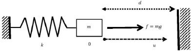
Figure 7.6. Situation of example 7.5
In this case,

Figure 7.7. Analysis of the situation of example 7.5
Let ![]() . Two situations are possible: if
. Two situations are possible: if ![]() , the external force f is small enough in order that the spring's force equilibrates f before the mass touches the obstacle and we have u = mg/k, so that DJ(u) = 0. If
, the external force f is small enough in order that the spring's force equilibrates f before the mass touches the obstacle and we have u = mg/k, so that DJ(u) = 0. If ![]() , the external force f is large enough in order to bring the mass to the contact with the obstacle. In this case, we have u = d, so that DJ(u) = kd – f < 0: in fact, the contact with the obstacle provokes a contact reaction R = mg – kd, which equilibrates the resulting force to zero.
, the external force f is large enough in order to bring the mass to the contact with the obstacle. In this case, we have u = d, so that DJ(u) = kd – f < 0: in fact, the contact with the obstacle provokes a contact reaction R = mg – kd, which equilibrates the resulting force to zero.
![]()
7.7. Lagrange’s multipliers
As shown in example 7.5, when constraints have to be taken into account, we have not DJ(u) = 0. In fact, we must introduce Lagrange’s multipliers λ in a penalty functional P(u; λ) and construct the Lagrangian L(u; λ) = J(u) + P(u; λ). These elements are defined according to the case under consideration:

We have:
Thus, (u; λ) is a saddle-point of L on V × Λ. Moreover, we have:
EXAMPLE 7.6 – Let us consider the situation of example 7.5. The constraint is I(u) = u – d ≤ 0. Thus, P(u; λ) = λI(u) = λ(u – d) and L(u; λ) = J(u) + λ(u – d). We have:
Moreover,
Thus,
and
So, the solution is given by:
![]()
EXAMPLE 7.7. – Let us consider an inextensible string of length ℓ > 0, linear mass density ρ > 0. Such a continuous medium is described by a ∈ (0, ℓ), where a is a particle of the string. Let us denote by u(a) the position of the particle a of the string: in a bidimensional approach, the position is a field u: (0, ℓ) → ![]() 2 and V = {v: (0, ℓ) →
2 and V = {v: (0, ℓ) → ![]() 2}. Since the string is inextensible, we have (u' = du/da)
2}. Since the string is inextensible, we have (u' = du/da)
Assume that the string is moored at the origin of the system of coordinates. We have also I1(u) = u1(0) = 0, I2(u) = u2(0) = 0. The energy of the string is the gravitational one:
Let us denote ![]() and
and ![]()
![]() . Observe that
. Observe that ![]() . Then,
. Then,
Thus,
So,
Using an integration by parts:

Thus,
λ1 is the tension, usually denoted by T, while t = u′(a) = u′(a)/|u'(a)| is the unitary tangent. The internal efforts are T = Tt. Thus, by denoting TO = λ2:

![]()
7.8. Primal and dual problems
Equation [7.1] shows that:
Thus, we may adopt two different approaches:
- 1) The first approach consists of determining u = argmin
 ,
,  and, then, find the Lagrange’s multipliers λ using the known u.
 - 2) The second approach consists of determining λ = argmax
 and, then, finding u using the knowns λ.
The first approach consists of solving the problem ![]() , which is referred to as the primal problem. The second one leads to the problem
, which is referred to as the primal problem. The second one leads to the problem ![]() , which is referred to as the dual problem.
, which is referred to as the dual problem.
The solution of the primal problem is usually performed by using standard optimization methods, such as penalty methods, projected gradient or reduced gradient methods etc. When considering the dual problem, the main approach is furnished by Uzawa’s method, which is a gradient’s method applied to the solution of the dual problem: at each iteration number n, λ(n–1) is given and we determine u(n–1) such that G(λ(n–1)) = L(u(n–1); λ(n–1)) Then, we determine an ascent direction d(n–1) (see Table 7.2).
Table 7.2. Ascent directions for Uzawa’s method

Given a fixed step μ > 0, we determine ![]() which completes the step. Then, we increase n and we pass to new iteration. The global algorithm for Uzawa’s method reads as:
which completes the step. Then, we increase n and we pass to new iteration. The global algorithm for Uzawa’s method reads as:
- 1) An initial guess λ(0), a fixed step μ > 0, a set of stopping conditions are given.
- 2) Set iteration number n ← 0.
- 3) Increase iteration number n ← n + 1.
- 4) Determine
 .
. - 5) Determine d(n–1).
- 6) Determine
 .
. - 7) Test for stopping conditions. If the decision is to continue the iterations, go to 3) or simply stop.
7.9. Matlab® determination of minimum energy solutions
The approximation of minimum energy solutions is performed according to the general principles presented in the preceding sections: we may consider a family ![]() and look for the unknowns U = (u1, … , uk). As previously, the coefficients are arranged in a matrix
and look for the unknowns U = (u1, … , uk). As previously, the coefficients are arranged in a matrix ![]() such that
such that ![]() In this case, we look for a minimum of:
In this case, we look for a minimum of:
Notice that U → u(U) is linear. Let us set δu = u(δU) = ![]() . We have:
. We have:
Then,
Let ![]() (k, n) be the set of the k × n real matrices. T:
(k, n) be the set of the k × n real matrices. T: ![]() (k, n) →
(k, n) → ![]() be given by:
be given by:
Since δu → DJ(u)(δu) is linear, we have:
Moreover, the linearity of T implies that:
We may evaluate ![]() by taking,
by taking,

Moreover,
so that:
Let us illustrate such an evaluation: let us assume that:
where fℓ is evaluated by the subprogram f_ell, while the gradient ![]() is evaluated by the subprogram gradf_ell. Then, J is evaluated by the subprogram
is evaluated by the subprogram gradf_ell. Then, J is evaluated by the subprogram
function v = functional(f_ell, u,a,b)
fff = @(t) f_ell(t, u(t));
xlim.lower.x = a;
xlim.upper.x = b;
xlim.dim = 1;
v = subprogram_integration(fff,xlim).result;
end
DJ may be evaluated as follows:
function v = der_functional(gradf_ell,u,du,a,b)
fff = @(t) dot(gradf_ell(t, u(t)),du(t));
xlim.lower.x = a;
xlim.upper.x = b;
xlim.dim = 1;
v = subprogram_integration(fff,xlim).result;
end
Jn and its gradient are evaluated as in section 7.5.3.
function v = jn(U,basis,J)
u = @(t) basis.projection(U,t);
v = J(u);
end
function v = gradjn(U,basis,dJ)
u = @(t) basis.projection(U,t);
v = zeros(size(U));
for j = 1: size(U,2)
    for p = 1: size(U,1)
        c = zeros(size(U));
        c(p,j) = 1;
        du = @(t) basis.projection(c,t);
        v(p,j) = dJ(u,du);
     end;
end;
For instance, let us consider:
a = 0;
b = 1;
f_ell = @(t,u) sum(u.^2);
gradf_ell = @(t,u) 2*u;
k = 3;
phi = polynomial_basis(0,a,b,k);
bp = basis(phi);
U = [0 0 ;
     0 1 ;
     1 0;
     0 0
     ];
J = @(u) functional(f_ell, u,a,b);
v = jn(U,bp,J)
dJ = @(u,du) der_functional(gradf_ell,u,du,a,b);
gv = gradjn(U,bp,dJ)
This code produces: v =0.4000 and
gv =
    0.6667   1.0000
    0.5000   0.6667
    0.4000   0.5000
    0.3333   0.4000
The exact value is ![]() ,
, ![]() , which is in accordance with the results obtained.
, which is in accordance with the results obtained.
Let us consider the unconstrained situation. In order to determine an approximate solution, we must find:
The evaluation of the gradient ![]() allows the use of gradient-based optimization methods for the minimization of Jn. As an example, let us consider the situation where:
allows the use of gradient-based optimization methods for the minimization of Jn. As an example, let us consider the situation where:
The exact solution is u1(t) = sin(t), u2(t) = cos(t). Let us consider the approximation by a polynomial family with = 5. We use f min search in order to minimize Jn. The results are exhibited in Figure 7.8.

Figure 7.8. Determination of the minimum of a functional
Let us consider the situation where constraints must be taken into account. As previously observed, we must consider a penalty functional P(u;λ) and the Lagrangian L(u; λ) = J(u) + P(u; λ). The primal problem may be solved by considering the penalty methods: a penalty function for the primal problem is a function p: V → ![]() such that p(u) = 0, if
such that p(u) = 0, if ![]() ; p(u) > 0, if
; p(u) > 0, if ![]() . A Typical penalty function for the constraint ψ(t, u(t)) ≤ 0 on Ω is:
. A Typical penalty function for the constraint ψ(t, u(t)) ≤ 0 on Ω is:
A typical penalty function for the constraint ψ(t, u(t)) = 0 on Ω is:
For the primal problem, sup{L(u; λ): λ} is attained for λ → + ∞, so that we may consider a fixed value λ > 0 and set Jλ(u) = L(u; λ) = J(u) + λp(u). Then, we determine:
This problem is unconstrained and may be solved by the preceding method. As an example, let us consider restrictions ![]() and
and ![]() . We assume that
. We assume that ![]() , and
, and ![]() , are evaluated by subprograms psineg, psieg, gradpsineg and gradpsieg, respectively. Then, we may evaluate the penalty by using the following subprogram:
, are evaluated by subprograms psineg, psieg, gradpsineg and gradpsieg, respectively. Then, we may evaluate the penalty by using the following subprogram:
function v = p_pen(u,lambda,psineg,psieg,a,b)
fff = @(t) penalty(t,u,psineg,psieg);
xlim.lower.x = a;
xlim.upper.x = b;
xlim.dim = 1;
v = subprogram_integration(fff,xlim).result;
v = lambda*v;
end
where:
function v = penalty(t,u,psineg,psieg)
aux = 0;
auxineg = psineg(t,u(t));
if ~isempty(auxineg)
    aux2 = (abs(auxineg)+auxineg)/2;
    aux = aux + sum(aux2.^2);
end;
auxeg = psieg(t,u(t));
if ~isempty(auxeg)
    aux = aux + sum(auxeg.^2);
end;
v = 0.5*aux;
return;
end
The Gâteaux differential of the penalty is evaluated as follows:
function v =
derp_pen(u,lambda,du,psineg,psieg,gradpsineg,gradps
ieg,a,b)
fff = @(t)
der_penalty(t,u,du,psineg,psieg,gradpsineg,gradpsie
g);
xlim.lower.x = a;
xlim.upper.x = b;
xlim.dim = 1;
v = subprogram_integration(fff,xlim).result;
v = lambda*v;
end
with
function v =
der_penalty(t,u,du,psineg,psieg,gradpsineg,gradpsieg)
aux = 0;
auxineg = psineg(t,u(t));
dauxineg = gradpsineg(t,u(t));
if ~isempty(auxineg)
    aux2 = (abs(auxineg)+auxineg)/2;
    aux =aux2'*dauxineg*du(t);
end;
auxeg = psieg(t,u(t));
dauxeg = gradpsieg(t,u(t));
if ~isempty(auxeg)
    aux = aux + auxeg'*dauxeg*du(t);
end;
v = aux;
return;
end
Let us consider:
function v = Jpen(u,lambda,J,P)
v = J(u) + P(u,lambda);
end
function v = der_Jpen(u,lambda,du,dJ,dP)
v = dJ(u,du) + dP(u,lambda,du);
end
We define the values of Jλ and DJλ as follows:
J = @(u) functional(f_ell, u,a,b);
P = @(u,lambda) p_pen(u,lambda,psineg,psieg,a,b);
Jlambda = @(u) Jpen(u,lambda,J,P);
dJ = @(u,du) der_functional(gradf_ell, u,du,a,b);
dP = @(u,lambda,du)
derp_pen(u,lambda,du,psineg,psieg,gradpsineg,gradps
ieg,a,b);
dJlambda = @(u,du) der_Jpen(u,lambda,du,dJ,dP);
Then, we may apply the method presented above for unconstrained situations. As an example, let us consider ![]()
![]() (no equality constraint), fℓ(t, u) = u1(t) – sin(t) + u2(t) – cos(t). The exact solution is u1(t) = sin(t), u2(t) = cos(t). Let us consider the approximation by a polynomial family with = 5. We use fminsearch in order to minimize Jn. The results are exhibited in Figure 7.9.
(no equality constraint), fℓ(t, u) = u1(t) – sin(t) + u2(t) – cos(t). The exact solution is u1(t) = sin(t), u2(t) = cos(t). Let us consider the approximation by a polynomial family with = 5. We use fminsearch in order to minimize Jn. The results are exhibited in Figure 7.9.

Figure 7.9. Determination of the unconstrained minimum of a functional
An alternative approach to primal problems is furnished by barrier methods: a barrier function is a function b: V → ![]() such that b(u) ∈
such that b(u) ∈ ![]() , if
, if ![]() ; b(u) = +∞, if
; b(u) = +∞, if ![]() and the penalty is P(u, λ) = λb(u). We do not develop this approach in this book, but the practical implementation is analogous to those of penalty methods.
and the penalty is P(u, λ) = λb(u). We do not develop this approach in this book, but the practical implementation is analogous to those of penalty methods.
For the dual problem, L(u;λ) = J(u) + P(u, λ) and we may use Uzawa’s algorithm. Let us split the vector λ in λ≤, λ=, corresponding to inequality and equality restrictions and stocked by variables lambineg,lambeg, respectively. Then, the penalty is evaluated as follows:
function v =
lag_pen(u,lambineg,lambeg,psineg,psieg,a,b)
fff = @(t)
lagpnlty(t,u,psineg,psieg,lambineg,lambeg);
xlim.lower.x = a;
xlim.upper.x = b;
xlim.dim = 1;
v = subprogram_integration(fff,xlim).result;
end
function v =
lagpnlty(t,u,psineg,psieg,lambineg,lambeg)
aux1 = 0;
aux2 = 0;
auxineg = psineg(t,u(t));
if ~isempty(auxineg)
   aux1 = lambineg(t)'*auxineg;
end;
auxeg = psieg(t,u(t));
if ~isempty(auxeg)
   aux2 = lambeg(t)'*auxeg;
end;
v = aux1 + aux2;
return;
end
The Gâteaux differential of the penalty is evaluated as follows:
function v =
derlag_pen(u,lambda,du,psineg,psieg,gradpsineg,grad
psieg,a,b)
fff = @(t)
der_lagpnlty(t,u,du,psineg,psieg,gradpsineg,gradpsi
eg);
xlim.lower.x = a;
xlim.upper.x = b;
xlim.dim = 1;
v = subprogram_integration(fff,xlim).result;
end
with
function v =
der_lagpntly(t,u,du,psineg,psieg,gradpsineg,gradpsi
eg)
auxineg = psineg(t,u(t));
dauxineg = gradpsineg(t,u(t));
if ~isempty(auxineg)
   aux1 = lambineg(t)'*dauxineg*du(t);
else
   aux1 = [];
end;
auxeg = psieg(t,u(t));
dauxeg = gradpsieg(t,u(t));
if ~isempty(auxeg)
   aux2 = lambeg(t)'*dauxeg*du(t);
else
   aux2 = [];
end;
if isempty(aux1)
v = aux2;
elseif isempty(aux2)
   v = aux1;
else
   v = aux1 + aux2;
end;
return;
end
Then, we evaluate the Lagrangian L(u; λ) as follows:
function v = Jpenlag(u,lambineg,lambeg,J,P)
v = J(u) + P(u,lambineg,lambeg);
end
function v =
der_Jpenlag(u,lambineg,lambeg,du,dJ,dP)
v = dJ(u,du) + dP(u,lambineg,lambeg,du);
end
In order to implement Uzawa’s method, we may use
J = @(u) functional(f_ell, u,a,b);
P = @(u,lambineg,lambeg)
lag_pen(u,lambineg,lambeg,psineg,psieg,a,b);
Jlambda = @(u) Jpenlag(u,lambineg,lambeg,J,P);
dJ = @(u,du) der_functional(gradf_ell, u,du,a,b);
dP = @(u,lambda,du)
derlag_pen(u,lambineg,lambeg,du,psineg,psieg,gradps
ineg,gradpsieg,a,b);
dJlambda = @(u,du)
der_Jplag(u,lambineg,lambeg,du,dJ,dP);
At each step of Uzawa’s method, we need to determine an unconstrained minimum of Jlambda and, then, use it to update the values of lambineg,lambeg. Uzawa’s iterations may be implemented as follows: the Lagrange’s multipliers are discretized on Ω = (a,b) by using a partition tp, such that a = tP1 < tp2 < … < tpn+1 = b. Table tp contains the values of these points tp(i) = tPi. The discrete values of the multipliers are stocked in the tables Lineg and Leg, with initial values Lineg0 and Leg0: Lineg(i) = λ≤ (tpi), Leg(i) = λ = (tpi). An initial guess U0 is given. Then, we use the code below:
Uopt = U0;
Lineg = Lineg0;
Leg = Leg0;
erruz = precuz + 1.;
nituz = 0;
while nituz < nituzmax && erruz > precuz
nituz=nituz+1;
if isempty(Lineg)
    lambineg = @(t) [];
else
    lambineg = @(t) interp1(tp,Lineg',t)';
end;
if isempty(Leg)
    lambeg = @(t) [];
else
    lambeg = @(t) interp1(tp,Leg',t)';
end;
   P = @(u, lambineg,lambeg)
lag_pen(u,lambineg,lambeg,psineg,psieg,a,b);
   Jlambda = @(u) Jpenlag(u, lambineg,lambeg,J,P);
   fobj = @(U) jn(U,bp,Jlambda);
   U_ini = Uopt;
   Uopt = fminsearch(fobj,U_ini);
   errineg = 0;
   if ~isempty(Lineg)
    auxineg = Lineg;
    for j=1:size(Lineg,2)
      aux = psineg(tp(j),u(tp(j)));
    for i = 1: size(Lineg,1)
      Lineg(i,j) = max([Lineg(i,j) + mu*aux(i),0]);
    end;
   end;
   errineg = norm(auxineg-Lineg);
end;
erreg = 0;
if ~isempty(Leg)
   auxeg = Leg;
   for j=1:size(Leg,2)
     aux = psieg(tp(j),u(tp(j)));
     for i = 1: size(Leg,1)
      Leg(i,j) = Leg(i,j) + mu*aux(i);
     end;
    end;
    erreg = norm(auxeg-Leg);
   end;
   erruz = errineg + erreg;
end;
As an example, let us consider ψ≤ (t, u(t)) = (sin(t) − u1(t), cos(t) − u2(t)), ψ = (x, u(x)) = [] (no equality constraint), fℓ(t, u) = |u(t)|2. The exact solution is u1(t) = max{sin(t),0}, u2(t) = max{cos(t),0}. Let us consider the approximation by a polynomial family with = 10. We use fminsearch in order to minimize Jn. The results are exhibited in Figure 7.10.

Figure 7.10. Determination of the constrained minimum of a functional by Uzawa’s method
7.10. First-order control problems
Differential equations may be used as constraints. For instance, let us consider the situation where:

This situation is referred to as first-order control problem: u is the control xa is the initial data and x is the state – it is determined by the control and the initial data. The differential equation is referred as state equation and J is usually called the cost functional. In this case, with λ = (λ1, λ2),
and

Thus,

which shows that (using integration by parts)

Moreover,

which shows that:
Finally, recall that:
Equations [7.2], [7.3] and [7.4] may be solved in order to determine the unknowns (x, u; λ). Notice that the approach presented in section 7.4.4 shows that:
This last equation is adequate for numerical solution: analogously to the situations examined in 7.9, we may consider a family F = {φi: 1≤ i ≤ k}, ![]() and look for the unknowns U = (u1, … , uk). In this case, we look for a minimum of:
and look for the unknowns U = (u1, … , uk). In this case, we look for a minimum of:
where x(U) is the solution of:
Let us use the same notation as in section 7.9:
Let δx be the solution of:
The gradient of Jn is evaluated analogously to section 7.9:
with
We have:

where ![]() and
and
In Matlab®, the state x may be determined as follows:
function x = state(fs,u,a,b,x0)
f = @(t,x) fs(t,x,u(t));
sol = ode45(f,[a,b],x0);
x = @(t) deval(sol,t);
end
δx may be evaluated as follows:
function dx = der_state(dfsdx,dfsdu,x,u,du,a,b,dx0)
df = @(t,dx) dfsdx(t,x(t),u(t))*dx +
dfsdu(t,x(t),u(t))*du(t);
sol = ode45(df,[a,b],dx0);
dx = @(t) deval(sol,t);
end
J may be evaluated as follows:
function v = functional(f,fs,u,a,b,x0)
x = state(fs,u,a,b,x0);
fff = @(t) f(t,x(t),u(t));
xlim.lower.x = a;
xlim.upper.x = b;
xlim.dim = 1;
v = subprogram_integration(fff,xlim).result;
end
DJ may be evaluated as follows:
function v =
der_functional(dfdx,dfdu,dfsdx,dfsdu,x,u,du,a,b,dx0)
dx = der_state(dfsdx,dfsdu,x,u,du,a,b,dx0);
fff = @(t)
dfdx(t,x(t),u(t))*dx(t)+dfdu(t,x(t),u(t))*du(t);
xlim.lower.x = a;
xlim.upper.x = b;
xlim.dim = 1;
v = subprogram_integration(fff,xlim).result;
end
Jn and its gradient are evaluated as in section 7.5.3.
function v = jn(U,basis,f,fs,a,b,x0)
u = @(t) basis.projection(U,t);
v = functional(f,fs,u,a,b,x0);
end
function v =
gradjn(U,basis,dfdx,dfdu,fs,dfsdx,dfsdu,a,b,x0,dx0)
u = @(t) basis.projection(U,t);
x = state(fs,u,a,b,x0);
v = zeros(size(U));
for i = 1: basis.nel
   du = @(t) basis.phi.value(i,t);
   v(i) =
der_functional(dfdx,dfdu,dfsdx,dfsdu,x,u,du,a,b,dx0);
end;
Let us illustrate the use of these equations by considering the situation where:
In this case,
In Matlab®, we define this situation as follows:
f = @(t,x,u) u.^2/(2*m) + alfa*abs(x) + h*x;
dfdu = @(t,x,u) u/m ;
dfdx = @(t,x,u) alfa*sign(x) + h;
fs = @(t,x,u) u;
dfsdu = @(t,x,u) 1 ;
dfsdx = @(t,x,u) 0;
The objective function is defined as:
fobj = @(U) jn(U,bp,f,fs,a,b,x0);
Its gradient is defined as:
gradfobj = @(U)
gradjn(U,bp,dfdx,dfdu,fs,dfsdx,dfsdu,a,b,x0,dx0);
We consider m = 1, g = 9.81, µ = 0.2, a = µmg, h = mg/2. The results furnished by a polynomial basis and by a trigonometrical basis (see section 2.2.6), both with k = 5, are shown in Figure 7.11.

Figure 7.11. Determination of a first-order control
7.11. Second-order control problems
The situation where

is referred to as second-order control problem. The approach presented in section 7.10 extends to this situation: here, λ =(λ1, λ2, λ3):

and

Thus,

In this case, an integration by parts furnishes:

These equations determine x and λ. Notice that the method presented in section 7.4.4 furnishes:
This situation may be reduced to the first-order control problem studied in section 7.10, by setting ![]() . Then:
. Then:

Thus, this problem may be solved by the approach introduced in section 7.10. Let us illustrate this approach by considering a linear oscillator:
Assume that we aim to force this oscillator to have a target phase: we look for the minimization of the objective
In this case,
which may be evaluated as follows:
fs = @(t,x,u)[x(2) ; u – c*x(2)/m – k*x(1)/m];
dfsdu = @(t,x,u) 1 ;
dfsdx = @(t,x,u)[-k/m, -c/m];
The objective corresponds to:
and may be defined as follows (om0 contains the value of ω0):
f = @(t,x,u) (x(1) - cos(om0*t)/om0)^2;
dfdu = @(t,x,u) 0 ;
dfdx = @(t,x,u) 2*[x(1) - cos(om0*t)/om0, 0];
The results obtained with m = 1, k = 1, c = 0, ![]() are shown in Figure 7.12.
are shown in Figure 7.12.

Figure 7.12. Determination of a first-order control
The results obtained with a polynomial family {<φi(t) = ti−1:1 ≤ i ≤ n}, n = 6, m = 1, k = 1, ![]() ,
, ![]() and 0.2, are shown in Figure 7.13.
and 0.2, are shown in Figure 7.13.

Figure 7.13. Second-order control: a linear oscillator
7.12. A variational approach for multiobjective optimization
Multiobjective optimization is often dated of the works of Francis Ysidro Edgeworth [EDG 81], which considers consumer decisions based on two utility functions – i.e. two objectives. Edgeworth pointed that the notion of optimum has no meaning in this situation, since the objectives may be contradictory. The reader may find in the literature the classical quote from Edgeworth about two objectives P and π ([EDG 81], p. 21):
It is required to find a point (x,y,) such that in whatever direction we take an infinitely small step, P and π do not increase together but that, while one increases, the other decreases.
With this phrase, Edgeworth introduces the idea of a trade-off between the objectives and defines the set nowadays known as Pareto Front, associated with Vilfredo Federico Damaso Pareto, born in Paris from a mixed French/Italian couple. Pareto introduced the notion of ophelimity – concurrent of that of utility – and defined the maximum ophelimity as the situation where it is impossible to make a small displacement (Pareto was civil engineer) in order that the ophelimity of each individual increases or decreases [PAR 06]. The book of Pareto was the sequence of his course held at the University of Lausanne [PAR 96, PAR 97]. His work was translated in French [PAR 09] and popularized in English [HIC 34a, HIC 34b], then translated into English [PAR 71].
The name of Pareto was associated with multiobjective optimization by means of Pareto Fronts and Pareto Efficiency. A recent work [ZID 14] proposed a variational method for the determination of Pareto fronts: assuming that both the objective functions are non-negative, we look for an admissible curve that minimizes the area between the curve and the vertical or horizontal axis (see Figure 7.7). We present below this approach for the situation where we are interested in minimizing two objective functions (f1(x), f2(x)), but the approach generalizes to vectors of objectives having larger dimension.
As previously observed, in the framework of multiobjective optimization, we are mainly interested in the determination of the Pareto front, i.e. the set of all the possible compromises between the different objectives. A Pareto front gives the possible trade-offs between the objectives and is formed by the non-dominated or efficient points. Let us recall that we may define a partial order on ![]() n as follows:
n as follows:
X ![]() Y ⇔ X
Y ⇔ X ![]() Y and there exists i ∈ {1, … , n} such that Xi < Yi.
Y and there exists i ∈ {1, … , n} such that Xi < Yi.
DEFINITION 7.4.– We say that X is more efficient than Y or that X dominates Y if and only if X ![]() Y.
Y.
Let S ⊂ ![]() n. We say that X is Pareto-efficient on S if and only if X ∈ S and there is no other element of S which is more efficient than X. The Pareto front or Pareto Frontier of S, denoted as ∏(S), is the set of the Pareto-efficients points of S:
n. We say that X is Pareto-efficient on S if and only if X ∈ S and there is no other element of S which is more efficient than X. The Pareto front or Pareto Frontier of S, denoted as ∏(S), is the set of the Pareto-efficients points of S:

Figure 7.14. Variational approach for multiobjective optimization (2 objectives)
Let ![]() .for 1 ≤ i ≤ n. The Pareto front associated with the vector of objectives f = (f1, … , fn) is ∏(S), where;
.for 1 ≤ i ≤ n. The Pareto front associated with the vector of objectives f = (f1, … , fn) is ∏(S), where;
Thus, the Pareto frontier is formed by the points X = (f1(x), … , fn(x)) such that there is not any y ∈ ![]() k such that
k such that ![]() verifies Y
verifies Y ![]() X.
X.
Let us apply these ideas to the situation where two objectives are under consideration (n = 2) and the Pareto front is defined by a function φ: ![]() 2 →
2 → ![]() that splits the plane in two disjoint regions, such that:
that splits the plane in two disjoint regions, such that:
The common boundary separating the two regions is:
Let us consider two points A ≠ B such that φ(A) = φ(B) = 0 (thus{A, B} ⊂ ∑). We consider the set:
Let us introduce a functional J: ℘ → ![]() such that:
such that:
Then
THEOREM 7.8.– Let P* = arg min {J(P): P ∈ ℘}. Then P*(t) ∈ ∑, for t ∈ (0,1).
![]()
PROOF.– Since P* ∈ ℘, we have φ(P*(t)) ≥ 0 on (0,1). Assume that there exists a point ![]() such that
such that ![]() . We have 0 < t < 1, since P*(0) = A ∈ ∑ and P*(1) = B ∈ ∑. Continuity of φ shows that there exists δ > 0 such that φ(P*(t)) > 0 for t ∈
. We have 0 < t < 1, since P*(0) = A ∈ ∑ and P*(1) = B ∈ ∑. Continuity of φ shows that there exists δ > 0 such that φ(P*(t)) > 0 for t ∈ ![]() . Let us consider the function:
. Let us consider the function:
We have:
Let
We have α(t)> 0, ![]() : indeed, if α(t) = 0, then there exists a sequence {αn: n ∈
: indeed, if α(t) = 0, then there exists a sequence {αn: n ∈ ![]() } such that αn > 0, ∀n and αn → 0 for n → +∞, with θ(αn, t) ≤ 0, i.e.
} such that αn > 0, ∀n and αn → 0 for n → +∞, with θ(αn, t) ≤ 0, i.e.
Taking the limit forn n → +∞, the continuity of φ shows that φ(P*(t)) ≤ 0. Thus, 0 < φ(P*(t)) = 0, which is a contradiction. Let us consider a regular function ![]() (0,1) such that ψ ≤ 0,
(0,1) such that ψ ≤ 0, ![]() and ψ(s) = 1 for s ∈ (a, b),
and ψ(s) = 1 for s ∈ (a, b), ![]() . ψ is extended by zero outside
. ψ is extended by zero outside ![]() and we define:
and we define:
On the other hand,
So that P ∈ ℘. On the other hand,
As a consequence, J(P) < J(P*). Or, P* = arg min{J(P): P ∈ ℘}, so that J(P*) ≤ J(P) < J(P*), which is a contradiction.
![]()
Corollary 7.2.– Let S ⊂ ![]() 2 be a non-empty closed set such that: ∃m ∈
2 be a non-empty closed set such that: ∃m ∈ ![]() : X1 ≥ m and X2 ≥ m,∀X = (X1, X2) ∈ S. Assume that S is regular in the sense that any continuous function defined on S has a continuous extension to
: X1 ≥ m and X2 ≥ m,∀X = (X1, X2) ∈ S. Assume that S is regular in the sense that any continuous function defined on S has a continuous extension to ![]() 2. Let,
2. Let,
Assume that ∑ is a curve P: (0,1) → ![]() 2 verifying P(0) = A, P(1) = B. Then,
2 verifying P(0) = A, P(1) = B. Then,
![]()
PROOF.– Let
We have φ(P) ≤ max {P1 − m, P2 − m}. In addition,
φ is continuous: indeed, if ||P − Q|| ≤ δ, then −δ ≤ P1 − Q1 ≤ δ and −δ ≤ P2− Q2 ≤ δ, so that:
Thus,
So, we have ![]() and φ is continuous. Let us extend φ by a regular function outside S: the result yields from the theorem.
and φ is continuous. Let us extend φ by a regular function outside S: the result yields from the theorem.
![]()
These results apply to the functional J defining the area between the horizontal axis and the curve.
For instance, we may use Stoke’s theorem: the circulation of a field of vectors ![]() along the closed curve
along the closed curve ![]() coincides with the flux of its rotational
coincides with the flux of its rotational ![]() on the surface
on the surface ![]() limited by the curve, i.e.,
limited by the curve, i.e.,
Let us consider a vector field ![]() such that
such that ![]() for a curb on the plane
for a curb on the plane ![]() . Then:
. Then:
For instance:
So, we may choose
In this case, the theorem and its corollary show that the solution is the curb P*(t): t ∈ (0,1) such that:

The second choice ![]() corresponds to a curve generated by a function P2 = η(P1). Then, P1(t) = t and P2 = η(t) = η(P1). The third choice
corresponds to a curve generated by a function P2 = η(P1). Then, P1(t) = t and P2 = η(t) = η(P1). The third choice ![]() corresponds a curve generated by a function P1 = η(P2). In this case, P2(t) = t and P1 = η(t) = n(P2).
corresponds a curve generated by a function P1 = η(P2). In this case, P2(t) = t and P1 = η(t) = n(P2).
EXAMPLE 7.8.– Let us consider ![]() . On (A, B): ν.dP = (P1P′2P′1)/2, so that:
. On (A, B): ν.dP = (P1P′2P′1)/2, so that:
We may simply look for P*(t): t ∈ (0,1) such that:
An alternative consists of setting
Then,
and
Under this formulation, we look for a curve x*(t): t ∈ (0,1) such that:

Euler–Lagrange's equations associated with this functional is:
where
We notice that δT(x) is a matrix. By rewriting:
We have:
i.e.
![]()
Example 7.9.– Let us consider ![]() . On
. On ![]()
![]() , so that:
, so that:
Thus, we may determine P*(t): t ∈ (0,1) such that:
We set, as in the preceding example,
Then,
and
In this case, we look for a curve bx*(t):t ∈ (0,1) such that:

The associated Euler–Lagrange's equation is:

where,
Analogously, rewriting:
we have:
i.e.
![]()
EXAMPLE 7.10- Let us consider ![]() on
on ![]()
![]() , so that:
, so that:
Here, we look for P*(t): t ∈ (0,1) such that:
with
We have:
and
In this case, we must determine a curve x* (t): t ∈ (0,1) such that:

The Euler–Lagrangr's equation because:
where,
Notice that δT (x) is a matrix. By rewriting:
we have:
i.e.
![]()
7.13. Matlab® implementation of the variational approach for biobjective optimization
Let us assume that the multiobjective optimization problem involves two functions f1, f2: ![]() n→
n→ ![]() . Let:
. Let:
In regular situations, the Pareto frontier is a curb connecting the points ![]() ,
, ![]() . Then, the Pareto front is given by (f1(x(t)), f2(x(t)): t ∈ (0,1).
. Then, the Pareto front is given by (f1(x(t)), f2(x(t)): t ∈ (0,1).
Let us introduce ![]() and χ(t) = x(t) − x0(t). χ verifies χ(0) = χ(1) = 0. Assuming differentiability, it becomes natural to look for
and χ(t) = x(t) − x0(t). χ verifies χ(0) = χ(1) = 0. Assuming differentiability, it becomes natural to look for ![]() . Thus, we may consider a family
. Thus, we may consider a family ![]() = {φi: 1 ≤ i ≤ k} and
= {φi: 1 ≤ i ≤ k} and ![]() . Then, we
. Then, we
look for the coefficients (χ1, … , χk) such that the area limited by the curve P(t) = (f_1(x°(t) + χtΦ), f2(x0 (t) + χtΦ)) is minimal.
We represent the problem in a Matlab® class biobjproblem., having properties as f1, f2, dim.:dim is an integer giving the dimension of the arguments of the objectives. f1, f2 are structures defining the objectives. Their properties are function and solution. The last property contains ![]() For instance, biobjproblem may be defined as follows:
For instance, biobjproblem may be defined as follows:
classdef biobjproblem
   properties
      f1
      f2
      dim
   end
   methods (Access = Public)
      function obj = biobjprob(f1,f2,dim)
         obj.f1 = f1;
         obj.f2 = f2;
         obj.dim = dim;
      end
   end
end
Let us consider a simple situation where n = 1, f1(x) = x2, f2(x) = (x − 1)2. We define:
f1.function = @(x) x^2;
f2.solution = 0;
f1.function = @(x) (x-1)^2;
f2.solution = 1;
dim = 1;
pb = biobjproblem(f1,f2,dim)
These commands create pb, containing the definitiion of the multiobjective problem. We define x0 as follows:
sol1 = pb.f1.solution;
sol2 = pb.f2.solution;
xzero = @(t) sol1 + t*(sol2 - sol1);
Let be given a vector χ and the family f as a basis. We generate a curb c as follows (tspan contains a partition of (0,1): for instance, tspan ![]()
functionp =
pareto_curb(chi,basis,xzero,problem,tspan)
c = @(t) basis.projection(chi,t) + xzero(t);
f1 = problem.f1.function;
f2 = problem.f2.function;
xa = zeros(problem.dim,length(tspan));
p1 = zeros(size(tspan));
p2 = zeros(size(tspan));
for i = 1: length(tspan);
xa(:,i) = c(tspan(i));
   p1(i) = f1(xa(:,i));
   p2(i) = f1(xa(:,i));
end;
p.x = p1;
p.y = p2;
p.curb = @(t) interp1(tspan,p.points,t);
return;
end
Assume that the area limited by the curve p.curb is evaluated by a subprogram surface(p). Then, our objective becomes to determine the coefficients chi that minimize
fobj = @(chi) pareto_surface(chi,basis,xzero,problem,tspan)
where,
function v = pareto_surface(chi,basis,xzero,problem,tspan)
p = pareto_curb(chi,basis,xzero,problem,tspan);
v = surface(p);
return;
end
In the examples below, surface(p) evaluates the surface by using a trapezoidal rule involving p.x. as horizontal data and p.y as vertical data. The Pareto front obtained in the simple situation is shown in Figure 7.15.

Figure 7.15. Variational approach for a simple biobjective optimization problem

Figure 7.16. Variational approach for a biobjective optimization problem
A more complex situation is shown in Figure 7.16, where are exhibited the results obtained for ![]()
![]() .
.
7.14. Exercises
EXERCISE 7.1.– Let ![]() be a regular bounded domain,
be a regular bounded domain,
with the scalar product
We assume that λ > 0, λ + 2μ ≥ 0. Let f = (f1, f2) ∈ [L2(Ω)]2, F(v) = (f, v)0 and J: V → R be given by
- 1) Show that

- 2) Determine DJ(u).
- 3) Let
 . Show that u∗ = u, where u is the solution of:

- 4) Show that J is strictly convex.
- 5) Conclude the uniqueness of u∗.
![]()
EXERCISE 7.2.– Let S = {v: (0,1) → ![]() : v(0) = 1, v(1) = 0}. Let J : S →
: v(0) = 1, v(1) = 0}. Let J : S → ![]() be a functional defined by
be a functional defined by ![]() . Let
. Let ![]()
- 1) Verify that S is an affine subspace.
- 2) Determine DJ(uε)(v).
- 3) Characterize uε as the solution of a variational equation.
- 4) Determine the differential equation and the boundary conditions satisfied by uε.
- 5) Show that uε does not exist.
![]()
EXERCISE 7.3.– Let S = {v: (0,1) → ![]() : v(0) = 1, v(1) = 0}. Let J: S →
: v(0) = 1, v(1) = 0}. Let J: S → ![]() be a functional defined by
be a functional defined by ![]()
![]()
- 1) Determine DJ(uε)(v).
- 2) Characterize uε as the solution of a variational equation.
- 3) Determine the differential equation and the boundary conditions satisfied by uε.
- 4) Determine uε.
- 5) Analyze the limit of uε for ε → 0 +.
![]()
EXERCISE 7.4.– Let ![]() . Let J : S →
. Let J : S → ![]() be a functional defined by
be a functional defined by ![]()
![]() .
.
- 1) Verify that S is an affine subspace.
- 2) Determine DJ(u)(v).
- 3) Characterize u as the solution of a variational equation.
- 4) Determine the differential equation and the boundary conditions satisfied by u.
![]()
EXERCISE 7.5.– Let ![]() . Let j : S →
. Let j : S → ![]() be a functional defined by
be a functional defined by ![]()
![]()
- 1) Verify that S is an affine subspace.
- 2) Determine DJ(u)(v).
- 3) Characterize u as the solution of a variational equation.
- 4) Determine the differential equation and the boundary conditions satisfied by u.
![]()
EXERCISE 7.6.– Find the curve defined by a function u: (0,1) → ![]() of fixed length ℓ > 0, such that u(0) = u(1) = 0, which maximizes the area limited by the curb and the horizontal axis. For instance, set
of fixed length ℓ > 0, such that u(0) = u(1) = 0, which maximizes the area limited by the curb and the horizontal axis. For instance, set ![]() and
and
Then,
- 1) Introduce the Lagrange multiplier η associated with Cand construct the Lagrangian L(u, η)associated with this problem;
- 2) Determine the Gâteaux derivative DuL;
- 3) Determine the differential equation and the boundary conditions satisfied by u;
- 4) Show that u defines an arc of circle.
![]()
EXERCISE 7.7.– Find the curve defined by a function u: (0,1) → ![]() connecting (0,0) and (1,0), such that it has the minimal length and respects an obstacle defined by a curb ψ: (0,1) →
connecting (0,0) and (1,0), such that it has the minimal length and respects an obstacle defined by a curb ψ: (0,1) → ![]() such that ψ(0) ≤ and ψ(1) ≤ 0.
such that ψ(0) ≤ and ψ(1) ≤ 0. ![]()
![]() . Then, minimize
. Then, minimize ![]() .
.
![]()
EXERCISE 7.8.– The motion of a point follows the equations:
Find the control u satisfying |u| ≤ 1 on (0, T) and x (T) = x1 for which T is minimal.
![]()
EXERCISE 7.9.– Let us consider the second-order system:
Find u such that 0 ≤ u ≤ 1 on (0, T), x(T) = x1, y(T) = y1 and ![]() dt is minimum (γ > 0, f known).
dt is minimum (γ > 0, f known).