
3
Hilbert Spaces for Engineers
David Hilbert is considered to be one of the most influential mathematicians of the 20th Century. He was a German mathematician, educated at Konigsberg, where he completed his PhD thesis under the direction of Ferdinand Lindemann. At the same time, Hermann Minkowski was also a PhD student of Lindemann – they presented their PhD’s in the same year (1885) and thereafter became good friends. Hilbert was acquainted with some of the best mathematicians of his time and contributed significantly to important mathematical problems. He also supported the candidacy of Emmy Noether to teach at the University of Gottingen – at these times, this university was considered one of the best mathematical centers of the world and women had difficulty in finding academic positions. The history of mathematics teems with anecdotes and quotes of Hilbert. At the 2nd International Congress of Mathematics held in Paris, in 1900, Hilbert presented a speech where he evoked unsolved problems. His speech was transcribed in a long article, first published in German, but which was quickly translated into English [WIN 02] and is known globally as the 23 Hilbert problems or the Hilbert program – this text has widely influenced Mathematics along the 20th Century. The Hilbert program addressed fundamental difficulties of Mathematics – some of them remain unresolved to this day – and their study led to a large development of new ideas and methods. For instance, the research connected to the second problem (the consistency of arithmetic) have led to the denial of any divine status to Mathematics and brought it to the dimension of a human activity based on human choices, biases and beliefs. The particularity of Mathematics remains in its quest for consistency and its extremely codified way to build results by logical deductions and demonstrations based on previous results. Mathematicians make choices by establishing axioms, which are the foundations of their buildings. Then, they patiently construct the whole structure by exploring the consequences of the axioms and generating results which are new bricks that make the building higher. The question of the compatibility of all the bricks among themselves is difficult and leads to the analysis of quality of the foundations, which is connected to the coherence of the results obtained, which may be weakened by paradoxes found in the development of the theory. The works of Kurt Godel [GOD 31] and Alfred Tarski [TAR 36] tend to show that we cannot be sure of the global compatibility of all the bricks and, so, of the coherence of the structure. But this apparent weakness transforms into force, since it gives power to imagination and total freedom for the construction of alternate theories, based on new axioms, which makes the possible developments of Mathematics virtually inexhaustible. This has led, for instance, to new geometries which have found applications in Physics and new function theories which have found their application in Physics and Engineering.
Ironically, Hilbert spaces were not formalized by Hilbert himself, but by other people. The three major contributions came from Maurice Fréchet [FRE 06], Stefan Banach [BAN 22] and John Von Neumann [VON 32]. Fréchet established a formalism based on the idea of distance in his PhD Thesis, prepared under the direction of Jacques Hadamard and presented in Paris in 1905. Banach presented the formalism of normed spaces in his PhD (1920 at Lvov), under the direction of Hugo Steinhaus – a former student of Hilbert. Banach also published an article presenting the formalization of normed spaces. Von Neumann worked with Hilbert and stated the axiomatic presentation of Hilbert spaces in his book. The original paper by Hilbert (the fourth of the series of six works on integral equations published between 1904 and 1910 [HIL 04a, HIL 04b, HIL 05, HIL 06a, HIL 06b, HIL 10, HIL 12] contains all the papers) did not present a formal theory and was limited to square summable functions [WEY 44].
In order to take the full measure of the importance of this work and the extent of its applications, the reader must recall that one of the main reasons for the existence of Mathematics is the need for the determination of the solutions of equations and the prediction of the evolution of systems or the determination of some of their parameters (namely, for safety or obtaining a desired result). Human activities often involve the generation of data, its analysis and conclusions about the future from observations or the determination of some critical parameters from data. This work is based on models representing the behavior of the system under analysis. However, the models involve equations that must be solved, either to generate the model or to determine the evolution of the system. For instance, Engineering and Physics use such an approach. Many of the interesting situations involve the solution of various types of equations (algebraic, differential, partial differential, integral, etc.). When studying integral, differential or partial differential equations, a major problem has to be treated, connected to the infinity: while the equation x ∈ ![]() and f(x) = 0 concerns a single value of x, the equation x(t) ∈
and f(x) = 0 concerns a single value of x, the equation x(t) ∈ ![]() and f(x(t),t) = 0, t ∈ (a, b) concerns infinite values of x (one for each t). Analogously, integral, differential or partial differential equations concern the determination of infinitely many values. Since the determination of infinite actions takes an infinite time, procedures like limits and approximations have been introduced. Instead of achieving an infinite amount of solutions, it seems more convenient to determine close approximations of the real solution by achieving a finite number of solutions.
and f(x(t),t) = 0, t ∈ (a, b) concerns infinite values of x (one for each t). Analogously, integral, differential or partial differential equations concern the determination of infinitely many values. Since the determination of infinite actions takes an infinite time, procedures like limits and approximations have been introduced. Instead of achieving an infinite amount of solutions, it seems more convenient to determine close approximations of the real solution by achieving a finite number of solutions.
The practical implementation of this simple idea begs answering some questions. For instance: what is the sense of “close”, i.e. who are the neighbors at a given distance of an element? How do we ensure that the approximations are close to “the real solution”, i.e. that there are neighbors of the real solution at an arbitrarily small distance? How do we obtain a sequence of solutions which are “closer and closer (i.e. convergent) to the real solution”, i.e. belonging to arbitrarily small neighborhoods of the real solution? Moreover, what is a solution? Mathematically, these questions may be formulated as follows: what is the set (x; ![]() ) = {y: distance between y and x≤ ε}? How do we ensure that an approximation
) = {y: distance between y and x≤ ε}? How do we ensure that an approximation ![]() verifies
verifies ![]() How do we generate an element xε
How do we generate an element xε ![]() V(x; ε) for an arbitrarily small ε > 0? By taking ε = 1/n and denoting xn = xε, this last question reads as: how to generate an element xn such that distance between xn and x ≤ 1/n, i.e. how do we generate a sequence {xn: n
V(x; ε) for an arbitrarily small ε > 0? By taking ε = 1/n and denoting xn = xε, this last question reads as: how to generate an element xn such that distance between xn and x ≤ 1/n, i.e. how do we generate a sequence {xn: n ![]()
![]() *} which converges to x? How do we define x into a convenient way?
*} which converges to x? How do we define x into a convenient way?
In the mathematical construction, elements such as the neighborhoods, the convergent sequences and approximations are defined by the topology of the space.
It is quite intuitive that we are interested in the construction of a theory and methods leading to the solution of the largest possible number of equations: for practical reasons, we want to be able to solve as many equations as possible. This means that we want to be able to generate the largest number of converging sequences {xn: n ∈ ![]() *} or, equivalently, that our main interest is the construction of spaces tending to include in the neighborhoods of given functions as many elements as possible (i.e. V(x; ε) is as large as possible).
*} or, equivalently, that our main interest is the construction of spaces tending to include in the neighborhoods of given functions as many elements as possible (i.e. V(x; ε) is as large as possible).
Increasing the members of a neighborhood, of solvable equations or of convergent sequences consists of weakening a topology: weaker topologies have more convergent sequences, more solvable equations and more elements in a neighborhood. But weaker topologies also introduce weaker regularity and a more complex behavior of the functions, so that a convenient topology establishes a balance between regularity and solvability.
In order to generate convenient topologies, we observe that Mathematics is constructed into a hierarchical way: the starting level is Set Theory, which defines objects that are mere collections and only involves operations such as intersection, union and difference.
In the next level, we consider operations involving the elements of the set itself: groups, rings, vectorial spaces. At this level, we have no concept of “neighbour”, “convergence” or “approximation”. In order to give a mathematical sense to these expressions, we need a topology.
A convenient way to define a topology consists of the introduction of a tool measuring the distance between two objects — i.e. a metric d(u, v)giving the distance between two elements u, v of the set (this was the work of Fréchet): then, we may define neighborhoods of u by considering the elements v such that d(u, v) ≤ ε, where ε is a small parameter: V(u; ε) = {v: d (u, v) ≤ ε}.
We may use a simple way to measure distances, which consists of using a norm ![]()
![]()
![]() measuring the “length” of the elements of V: d(u, v) =
measuring the “length” of the elements of V: d(u, v) = ![]() u − v
u − v![]() , i.e. the distance between u and v is measured as the length of the difference between the elements u, v (this was the work of Banach).
, i.e. the distance between u and v is measured as the length of the difference between the elements u, v (this was the work of Banach).
The next level consists of introducing a measure of the angle between the elements u, v − this is made by using the scalar product (u, v) and was the work of Von Neumann. We will see that such a structure has more complex neighbourhoods and leads to a larger number of converging sequences. Thus, this last level leads to more converging sequences, more complete neighborhoods and gives at the same time measures of angles, lengths and distances. It corresponds to Hilbert Spaces and furnishes an interesting framework for the definition of convenient topologies.
3.1. Vector spaces
Vector spaces are a fundamental structure for variational methods. The definition of a vector space assumes that two sets were defined: a set Λ of scalars and a set V of vectors. The set of scalars is usually the set of real numbers ![]() or the set of complex numbers
or the set of complex numbers ![]() — even if, in general, we may consider any field, i.e. any algebraical structure having operations of addition and multiplication with their inverses (subtraction and division). In the sequel, we consider vector spaces on
— even if, in general, we may consider any field, i.e. any algebraical structure having operations of addition and multiplication with their inverses (subtraction and division). In the sequel, we consider vector spaces on ![]() , i.e. we assume that Λ =
, i.e. we assume that Λ = ![]() . However, in a general approach, V may appear as arbitrary, but in our applications V will be a functional space, i.e. the elements of V will be considered as functions. The formal definition of a vector space on
. However, in a general approach, V may appear as arbitrary, but in our applications V will be a functional space, i.e. the elements of V will be considered as functions. The formal definition of a vector space on ![]() (resp. Λ) assumes that V possesses two operations: addition u + v of two elements u, v ∈ and multiplication λu of an element u of V by a scalar λ∈
(resp. Λ) assumes that V possesses two operations: addition u + v of two elements u, v ∈ and multiplication λu of an element u of V by a scalar λ∈ ![]() (respectively, Λ). Then,
(respectively, Λ). Then,
DEFINITION 3.1.– Let V ≠ ∅ be such that:

Then, V is a vector space on ![]() .
.
![]()
We have:
THEOREM 3.1.— Let V be a vector space space on ![]() and S ⊂ V. S is a vector space on
and S ⊂ V. S is a vector space on ![]() if and only if 0 ∈ S and λu + v ∈ V, ∀λ ∈
if and only if 0 ∈ S and λu + v ∈ V, ∀λ ∈ ![]() u, v ∈ S. ∈ In this case, S is said to be a vector subspace of V.
u, v ∈ S. ∈ In this case, S is said to be a vector subspace of V.
PROOF.– We have(−l)u + 0 = −u(see exercises). Thus, −u ∈ S, ∀ u ∈ S. Thus, all the conditions of definition 3.1 are satisfied by S.
EXAMPLE 3.1.— Let us consider Ω ⊂ ![]() n and V = {v: Ω →
n and V = {v: Ω → ![]() k}. V is a vector space on
k}. V is a vector space on ![]() (see exercises). Thus any subset of V such that 0 ∈ S and λu + v ∈ V, ∀λ ∈
(see exercises). Thus any subset of V such that 0 ∈ S and λu + v ∈ V, ∀λ ∈ ![]() , u, v ∈ S is also a vector space on
, u, v ∈ S is also a vector space on ![]() . For instance:
. For instance:

are both vector subspaces of V.
![]()
DEFINITION 3.2.— Let F = {φλ: λ ∈ Λ} ⊂ V, Λ ≠ ø, F ≠ ø. F is linearly independent (or free) if and only if a finite linear combination ![]() of its elements is null if and only if all the coefficients ai are null
of its elements is null if and only if all the coefficients ai are null
We denote by [F ] the set of the finite linear combinations of elements of F:
We say that F is a generator (or that F spans V) if and only if [F] = V. We say that F is a basis of F if and only if F is free and Fspans V. The number of elements of the basis is the dimension of V: if the basis contains n elements, we say that V is n-dimensional (ordim (V) = n); if V contains infinitely many elements, we say that V is infinite dimensional (or dim(V) = +∞).
![]()
Any vector space containing at least one element non null has a basis (see [SOU 10]). In the following, we are particularly interested in countable families F, i.e. in the situations where Λ = ![]() *. We will extend the notion of “basis” to the notion of “Hilbert basis”, where we have not if [F] = V, but V is the limit of elements of [F].
*. We will extend the notion of “basis” to the notion of “Hilbert basis”, where we have not if [F] = V, but V is the limit of elements of [F].
3.2. Distance, norm and scalar product
The structure of a vector space does not contain elements for the definition of neighbors, i.e. does not allow us to give a sense to the expressions “close to” and “convergent”. In order to give a practical content to these ideas, we must introduce new concepts: the distance between elements of V, the norm of an element of V, the scalar product of elements of V.
3.2.1. Distance
The notion of distance allows the definition of neighbors and quantifies as far or as close are two elements.
DEFINITION 3.3.– Let d: V × V → ![]() be a function such that
be a function such that

Then, d is a distance on V.
As previously observed, we are not interested in the numeric value of a distance, but in the definition of families of neighbors in order to approximate solutions and study convergence of sequences. For such a purpose, the numeric value of a distance is not useful as information. For instance, if d is a distance on V and η: ![]() →
→![]() is a strictly increasing application such that η(0) = 0 and η(a + b) ≤ η(a) + η(b), then dη,(u, v) = η(d(u, v)) is a distance on V (see exercises). Thus, we may give an arbitrary value to the distance between two elements of V. Moreover, distances may be pathological: for instance, the defination
is a strictly increasing application such that η(0) = 0 and η(a + b) ≤ η(a) + η(b), then dη,(u, v) = η(d(u, v)) is a distance on V (see exercises). Thus, we may give an arbitrary value to the distance between two elements of V. Moreover, distances may be pathological: for instance, the defination
corresponds to a distance. This distance is not useful, since the small neigborhoods of u contain a single element, which is u itself: d(u, v)≤ ε ≤1 ⇒ v = u. Thus, V(u; ε) = {u} and the associated topology contains just a few converging sequences and neighborhoods are poor in elements.
Distances allow the definition of limits and continuity. Since our presentation focuses on Hilbert spaces, these notions are introduced later, when considering norms.
3.2.2. Norm
The notion of norm allows the definition of the length of a vector and, at the same time, may be used in order to define a distance. In Mechanics, norms may also be interpreted in terms of internal energy of a system.
DEFINITION 3.4.– Let ![]()
![]()
![]() : V →
: V → ![]() be a function such that
be a function such that

Then, ![]()
![]()
![]() is a norm on V.
is a norm on V.
![]()
Classical examples of norms on V = ![]() n are (x = (x1, …, x„)):
n are (x = (x1, …, x„)):
THEOREM 3.2.– Let ![]()
![]()
![]() be a norm on V. Then d(u, v) =
be a norm on V. Then d(u, v) = ![]() u − v
u − v ![]() is a distance on V.
is a distance on V.
![]()
PROOF.– Immediate.
![]()
When considering functional spaces, such as subspaces of V = {v: Ω ⊂ ![]() n →
n → ![]() k} continuity may be an essential assumption in order to define norms. For instance, let us consider p ∈
k} continuity may be an essential assumption in order to define norms. For instance, let us consider p ∈ ![]() * and
* and
Let S = {v ∈ V: v is continuous on Ω and ![]() v
v![]() < ∞ }, then
< ∞ }, then ![]()
![]()
![]() is a norm on S. The assumption of continuity is used in order to show that
is a norm on S. The assumption of continuity is used in order to show that
Indeed, for v continuous on Ω:
If x ∈ Ω is such that ![]() v(x)
v(x)![]() p > 0, the, by continuity, there is ε > 0 such that
p > 0, the, by continuity, there is ε > 0 such that ![]() v(y)
v(y)![]() p>0 on Bε(x) = {y ∈ Ω:
p>0 on Bε(x) = {y ∈ Ω: ![]() y − x
y − x![]() ≤ ε} (Corollary 3.1). Then,
≤ ε} (Corollary 3.1). Then,
and we have 0 > 0, what is a contradiction. The classical counterexample establishing that continuity must be assumed is furnished by a function v such that v(x) = 0 everywhere on Ω, except on a finite or enumerable number of points. For instance,
Here, ![]() v
v ![]() = 0, but v≠ 0. In the following, we show how to we lift this restriction by using equivalence relations that generate the functional space Lp(Ω) − there will be a price to pay: it will be the loss of the concept of value at a point: the individual value v (x) of v in a point x has no meaning for elements of Lp(Ω).
= 0, but v≠ 0. In the following, we show how to we lift this restriction by using equivalence relations that generate the functional space Lp(Ω) − there will be a price to pay: it will be the loss of the concept of value at a point: the individual value v (x) of v in a point x has no meaning for elements of Lp(Ω).
As an alternative norm, we may also consider
In this case, the assumption of continuity is not necessary. Indeed,
3.2.3. Scalar product
The notion of scalar product allows the definition of angles between vectors and, at same time, may be used in order to define a norm. In Mechanics, scalar products may also be interpreted as the virtual work of internal efforts.
DEFINITION 3.5.– Let (![]() ,
, ![]() ): V × V →
): V × V → ![]() be a function such that
be a function such that

Then, (![]() ,
, ![]() ) is a scalar product on V.
) is a scalar product on V.
![]()
A classical example of scalar product on V = ![]() n is (x = (x1, …, xn), y = (y1, …, yn))
n is (x = (x1, …, xn), y = (y1, …, yn))
THEOREM 3.3.– Let (![]() ,
, ![]() ): V × V →
): V × V → ![]() be a scalar product on V. Then, ∀u, v, ∈ V, λ ∈
be a scalar product on V. Then, ∀u, v, ∈ V, λ ∈ ![]() ,
,
- i)

- ii)

- iii)

- iv)

- v)

- vi)

![]()
PROOF— We have
so that,
and we have (i). Thus:
By adding these two equalities, we have (ii).
Let f(λ) = (u + λv, u + λv). We have f(λ) ≥ 0, ∀λ ≥ 0. Thus,
and we have (iii).
Since
We have
what implies (iv). Replacing v by − v, we obtain (v).
Finally, we observe that
so that (from(iii))
and we have (vi).
![]()
THEOREM 3.4.— Let (![]() ,
, ![]() ): V × V →
): V × V → ![]() be a scalar product on V. Then,
be a scalar product on V. Then, ![]() is a norm on V.
is a norm on V.
![]()
PROOF — we have

Finally, 3.2.5. (v) implies that ![]() u + v
u + v![]() ≤
≤ ![]() u
u![]() +
+ ![]() v
v![]() .
.
Functional spaces, such as subspaces of ![]() generally involve continuity assumptions in order to define scalar products. Analogously to norms, the assumption of continuity is necessary in order to verify that
generally involve continuity assumptions in order to define scalar products. Analogously to norms, the assumption of continuity is necessary in order to verify that
For instance, if
and S = {v ∈ V: v is continuous on Ω and (y, v) < ∞}, then (![]() ,
, ![]() ) defines a scalar product on S. Analagously to the case of norms (use p = 2),
) defines a scalar product on S. Analagously to the case of norms (use p = 2),
In the following, continuity assumption is lifted by using functional space L2(Ω). As previously observed, the consequence is the loss of the meaning of point values v(x)
This limitation may be avoided in particular situations where the scalar product implies the continuity. For instance, let us consider,
where A: B = Σi, j Aij Bij. In this case, the continuity of the elements u, v yields from , the existence of the gradients ∇u, ∇v and we may give a meaning to the punctual values u(x) and (x) .
DEFINITION 3.6.— The angle θ(u, v) between the vectors u and v is
u and v are orthogonal if and only if (u, v) = 0 Notation: u ⊥v. For S ⊂ V, we denote by S⊥ the set of the elements of V which are orthogonal to all the elements of S:
![]()
DEFINITION 3.7.– Let F = {φn : n ∈ Λ ⊂ ![]() *} be a countable family. We say that F is an orthogonal family if and only if
*} be a countable family. We say that F is an orthogonal family if and only if
We say that F is an orthonormed family if and only if it is orthogonal and, moreover,
![]()
A countable free family G = {øn: n ∈ Λ ⊂ ![]() *} may be transformed into an orthonomal family F = {φn: n ∈ Λ ⊂
*} may be transformed into an orthonomal family F = {φn: n ∈ Λ ⊂ ![]() *} by the Gram–Schmidt procedure, which has been created for the solution of least-square linear problems. It has been proposed by Jorgen Pedersen Gram [GRA 83] and formalized by Ehrlich Schmidt [SCM 07] (although early uses by Pierre Simon de Laplace have been noticed [LEO 13]). The Gram–Schmidt procedure reads as:
*} by the Gram–Schmidt procedure, which has been created for the solution of least-square linear problems. It has been proposed by Jorgen Pedersen Gram [GRA 83] and formalized by Ehrlich Schmidt [SCM 07] (although early uses by Pierre Simon de Laplace have been noticed [LEO 13]). The Gram–Schmidt procedure reads as:
- 1) Set

- 2) For k > 0, set

In this case,
The practical implementation requests the evaluation of scalar products and norms.
As an example, let us consider Ω = (−1, 1) and
The family øn(x) = xn is not orthonormal, since (mod(p, q) denotes the remainder of the integer division p/q)
If the Gram–Schmidt procedure is applied, we have:
3.2.4. Cartesian products of vector spaces
In practice, we often face situations where V = V1 × … Vd is the Cartesian product of vector spaces. In this case, elements u, ![]() are given by:
are given by:
In such a situation:
- – If the distance on Vi is di, then the distance d„ on V may be defined as:

- – Analogously, if the norm on Vt is

 , then the norm v on V may be dfined as:
- – Finally, if the scalar product on Vi is (, )i, then the scalar product (, )v on V may be defined as:

When
 , we have
  and
and
3.2.5. A Matlab® class for scalar products and norms
Below we give an example of a Matlab® class for the evaluation of scalar products and norms. The class contains two scalar products:
Evaluated by methods sp0 and sp1, respectively. The associated norms are evaluated by methods n0 and n1, respectively. For each method, the functions are furnished by structured data. In both the cases, the structure has as properties dim, dimx and component. dim and dimx are integer values defining the dimension of the function and the dimension of its argument x. component is a cell array of length dim containing the values of the components and their gradients: each element of component is a structure having properties value and grad. When using ‘subprogram’, value and grad are Matlab subprograms (i.e. anonymous functions). For ‘table’, value is an array of values and grad is a cell arrays containing tables of values: u.component{i}.value is a table of values of component ui; and u. component {i} .grad {j} is a table of values of ∂ui/∂xj.
For ‘subprogram’, parameter xl contains the limits of the region, analogous to those used in class subprogram_integration. For ‘table’, xl is a structure containing the points of integration, analogously to those used in class riemann.
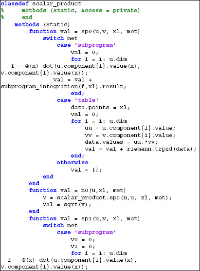

Program 3.1. A class for the determination of partial solutions of linear systems
EXAMPLE 3.2.– Let us evaluate both the scalar products and norms for the functions u, v: (0, 1) → ![]() given by u(x) = x, v(x) = x2. The functions may be defined as follows:
given by u(x) = x, v(x) = x2. The functions may be defined as follows:

Program 3.2. Definition of u and v in example 3.2
The code:
xlim.lower.x = 0;
xlim.upper.x = 1;
xlim.dim = 1;
u = u1();
v = v1();
sp = scalar_product();
sp0uv = sp.sp0(u,v, xlim,‘subprogram’);
n0u = sp.n0(u,xlim,‘subprogram’);
n0v = sp.n0(v,xlim,‘subprogram’);
sp1uv = sp.sp1(u,v, xlim,‘subprogram’);
n1u = sp.n1(u,xlim,‘subprogram’);
n1v = sp.n1(v,xlim,‘subprogram’);
produces the results sp0uv = 0.25, n0u = 0.57735, n0v = 0.44721, sp1uv = 1.25, n1u = 1.1547, n1v = 1.2383.
The exact values are, respectively, ![]()
![]()
We generate cell arrays containing tables of values by using:
x = 0:0.01:1;
p.x = x;
p.dim = 1;
U.dim = 1;
U.dimx = 1;
U.component = cell(u.dim,1);
U.component{1}.value =
spam.partition(u.component{1}.value,p);
U.component{1}.grad = cell(u.dim,1);
U.component{1}.grad{1} =
spam.partition(u.component{1}.grad,p);
V.dim = 1;
V.dimx = 1;
V.component = cell(v.dim,1);
V.component{1}.value =
spam.partition(v.component{1}.value,p);
V.component{1}.grad = cell(v.dim,1);
V.component{1}.grad{1} =
spam.partition(v.component{1}.grad,p);
Then, the code:
sp0UV = sp.sp0(U,V,p,'table');
n0U = sp.n0(U,p,'table');
n0V = sp.n0(V,p,'table');
sp1UV = sp.sp1(U,V,p,'table');
n1U = sp.n1(U,p,'table');
n1V = sp.n1(V,p,'table');
produces the results sp0UV = 0.25003, n0U = 0.57736, n0V = 0.44725, sp1UV = 1.25, n1U = 1.1547, n1V = 1.2383.
![]()
EXAMPLE 3.3.— Let us evaluate both the scalar products and norms for the functions u, v: (0, 1) × (0, 2) → ![]() given by
given by ![]()
![]() . The functions may be defined as follows:
. The functions may be defined as follows:

Program 3.3. Definition of u and v in example 3.3
The code:
xlim.lower.x = 0;
xlim.upper.x = 1;
xlim.lower.y = 0;
xlim.upper.y = 2;
xlim.dim = 2;
u = u2();
v = v2();
sp = scalar_product();
sp0uv = sp.sp0(u,v, xlim,'subprogram');
n0u = sp.n0(u,xlim,'subprogram');
n0v = sp.n0(v,xlim,'subprogram');
sp1uv = sp.sp1(u,v, xlim,'subprogram');
n1u = sp.n1(u,xlim,'subprogram');
n1v = sp.n1(v,xlim,'subprogram');
produces the results sp0uv = 1.8333, n0u = 0.94281, n0v = 2.0976, sp1uv = 4.8333, n1u = 2.0548, n1v = 3.0111.
The exact values are, respectively ![]()
We use the function
function v = select_index(ind,u,x)
aux = u(x);
v = aux(ind);
return;
end
and we generate cell arrays containing tables of values by the code below:
x = 0:0.01:1;
y = 0:0.01:2;
p.x = x;
p.y = y;
p.dim = 2;
U.dim = 1;
U.dimx = 2;
U.component = cell(u.dim,1);
U.component{1}.value =
spam.partition(u.component{1}.value,p);
U.component{1}.grad = cell(u.dim,1);
V.dim = 1;
V.dimx = 2;
V.component = cell(u.dim,1);
V.component{1}.value =
spam.partition(v.component{1}.value,p);
V.component{1}.grad = cell(u.dim,1);
for i = 1: u.dim
  for j = 1: p.dim
    du = @(x) select_index(j,u.component{i}.grad,x);
    U.component{i}.grad{j} = spam.partition(du,p);
    dv = @(x) select_index(j,v.component{i}.grad,x);
    V.component{i}.grad{j} = spam.partition(dv,p);
  end;
end
sp0UV = sp.sp0(U,V,p,'table');
n0U = sp.n0(U,p,'table');
n0V = sp.n0(V,p,'table');
sp1UV = sp.sp1(U,V,p,'table');
n1U = sp.n1(U,p,'table');
n1V = sp.n1(V,p,'table');
It produces the results sp0UV = 1.8334, n0U = 0.94284, n0V = 2.0977, sp1UV = 4.8334, n1U = 2.0548, n1V = 3.0111.
![]()
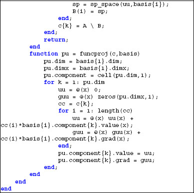
3.2.6. A Matlab® class for Gram–Schmidt orthonormalization
The class defined in the preceding section may be used in order to transform a general family G = {øi: 1 ≤ i ≤ n} into an orthonomal family F = {φi: 1 ≤ i ≤ n} by the Gram–Schmidt procedure.
Let us assume that the family G is defined by a cell array basis such that basis{i} defines øi, according to the standard defined in section 3.2.5 : basis{i} is a structure having properties dim, dimx and component. component is a structure having fields value and grad. The class given in program 3.4 generates a cell array hilbert_basis defining the family F, resulting from the application _ the Gram–Schmidt’s procedure to G. The class uses subprograms sp_space and n_space, which are assumed to evaluate the scala product and the norm.


Program 3.4. A class for the Gram-Schmidt orthogonalization
EXAMPLE 3.4.— Let us consider the family øi(x) = xi−1

Program 3.5. Definition of the family G in example 3.4
The family is created by the code
basis = cell(n,1);
for i = 1: n
  basis{i} = u3(i);
end;
We apply the procedure on (−1, 1) with the scalar product sp0:
xlim.lower.x = -1;
xlim.upper.x = 1;
xlim.dim = 1;
sp_space = @(u,v)
scalar_product.sp0(u,v,xlim,'subprogram');
n_space = @(u)
scalar_product.n0(u,xlim,'subprogram');
hb =
gram_schmidt.subprograms(basis,sp_space,n_space);
The results are shown in Figure 3.1 below:

Figure 3.1. Results for example 3.4 (using sp0 and ‘subprograms’). For a color version of the figure, see www.iste.co.uk/souzadecursi/variational.zip
We generate discrete data associated with these functions by using the code:
x = -1:0.02:1;
p.x = x;
p.dim = 1;
tb = cell(n,1);
for i = 1: n
  u = u3(i);
  U.dim = 1;
U.dimx = 1;
  U.component = cell(u.dim,1);
  U.component{1}.value =
spam.partition(u.component{1}.value,p);
  U.component{1}.grad = cell(u.dim,1);
  U.component{1}.grad{1} =
spam.partition(u.component{1}.grad,p);
  tb{i} = U;
end;
Then, the commands
sp_space = @(u,v)
scalar_product.sp0(u,v,p,'table');
n_space = @(u) scalar_product.n0(u,p,'table');
hb = gram_schmidt.tables(tb,sp_space,n_space);
furnish the result shown in Figure 3.2 below:

Figure 3.2. Results for example 3.4 (using sp0 and ‘tables’). For a color version of the figure, see www.iste.co.uk/souzadecursi/variational.zip

Figure 3.3. Results for example 3.4 using sp1 and ‘subprograms’. For a color version of the figure, see www.iste.co.uk/souzadecursi/variational.zip

Figure 3.4. Results for example 3.4 using sp1 and ‘tables’. For a color version of the figure, see www.iste.co.uk/souzadecursi/variational.zip
When the procedure is applied with the scalar product sp1, the results differ. For instance, we obtain the results exhibited in Figures 3.3 and 3.4:
As an alternative, we may define the basis by using the classes previously introduced (section 2.2.6). For instance,
zero = 1e-3;
xmin = -1;
xmax = 1;
degree = 3;
bp = polynomial_basis(zero,xmin,xmax,degree);
%
basis = cell(n,1);
for i = 1: n
  basis{i}.dim = 1;
  basis{i}.dimx = 1;
  basis{i}.component = cell(1,1);
  basis{i}.component{1}.value = @(x) bp.value(i,x);
  basis{i}.component{1}.grad = @(x) bp.d1(i,x);
end;
This definition leads to the same results.
![]()
3.3. Continuous maps
As previously indicated, distances allow the introduction of the concept of continuity of a function. For a distance defined by a norm (as in theorem 3.2),
DEFINITION 3.8.– Let V, W be two vector spaces having norms ![]()
![]()
![]() v,
v, ![]()
![]()
![]() w, respectively. Let T: V → W be a function. We say that T is continuous at the point u ∈ V if and only if
w, respectively. Let T: V → W be a function. We say that T is continuous at the point u ∈ V if and only if
We say that T is continuous on A ⊂ V if and only if ∀u ∈ A : T is continuous at u.
We say that T is uniformly continuous on A ⊂ V if and only if δ is independent of u on A: δ(u, ε) = δ(ε), ∀u ∈ A.
![]()
An example of uniformly continuous function is T: V → ![]() given by T(u) =
given by T(u) = ![]() u
u![]() : we have
: we have ![]()
![]() u
u![]() −
− ![]() v
v![]()
![]() ≤
≤ ![]() u − v
u − v![]() so that δ(u, ε) = ε.
so that δ(u, ε) = ε.
Continuous functions have remarkable and useful properties. For instance,
PROPOSITION 3.1.— Let V be a vector space having norm![]()
![]()
![]() . Let T: V →
. Let T: V → ![]() be continuous at the point u ∈ V. If T(u) > 0 (resp. (u)< 0), then there exists δ > 0 such that
be continuous at the point u ∈ V. If T(u) > 0 (resp. (u)< 0), then there exists δ > 0 such that
![]()
PROOF.– Take ε = ![]() T(u)
T(u)![]() /2 and δ = δ(u, e). From definition 3.5,
/2 and δ = δ(u, e). From definition 3.5,
and we have the result stated.
![]()
COROLLARY 3.1.— Let V, W be two vector spaces having noms![]()
![]()
![]() v,
v,![]()
![]()
![]() w, respectively. Let F:V→ W be continuous at the point u ∈ V. If F(u) ≠ 0 then there exists δ > 0 such that
w, respectively. Let F:V→ W be continuous at the point u ∈ V. If F(u) ≠ 0 then there exists δ > 0 such that
![]()
PROOF.– Since F is continuous at u,
Let T(v) = ![]() F(v)
F(v)![]() w. We have
w. We have
therefore, that T is continuous at u and the result follows from proposition 3.1.
![]()
3.4. Sequences and convergence
Our main objective is the determination of numerical approximations to equations (algebraic, differential, partial differential, etc.). Approximations are closely connected to converging sequences.
3.4.1. Sequences
DEFINITION 3.9.— A sequence of elements of V (or a sequence on V) is an application ![]() *∋n → un ∈ V. Such a sequence is denoted {un: n ∈ W} ⊂ V .
*∋n → un ∈ V. Such a sequence is denoted {un: n ∈ W} ⊂ V .
Let ![]() * ∋ k → nk ∈
* ∋ k → nk ∈ ![]() * be a strictly increasing map. Then
* be a strictly increasing map. Then ![]() * ∋
* ∋ ![]() ∈ V is a subsequence
∈ V is a subsequence ![]() ⊂ {un: n ∈
⊂ {un: n ∈![]() *}
*}
![]()
We observe that nk → +∞ when k → +∞ : we have nk+1 > nk so that nk+1 ≥nk + l. Thus, nk+1 ≥ n1+ k≥k and nk → +∞ .
In the context of engineering, the main interest of sequences the main interest lies in their use in the construction of approximations, whether for functions (for instance, signals) or solutions of equations. Approximations are connected to the notion of convergence. In the following, we present this concept and we distinguish strong and weak convergence.
3.4.2. Convergence (or strong convergence)
DEFINITION 3.10.– Let V be a vector space having norm ![]()
![]()
![]() . {un: n ∈
. {un: n ∈ ![]() *} ⊂ V converges (or strongly converges) to u ∈ V if and only if
*} ⊂ V converges (or strongly converges) to u ∈ V if and only if ![]() un − u
un − u![]() → 0, when n → ∞. Notation: un → u or u = limn→ +∞ un.
→ 0, when n → ∞. Notation: un → u or u = limn→ +∞ un.
![]()
EXAMPLE 3.5.— Let us consider un: (0,1) → ![]() given by
given by

and

We have

Thus, un → u on V = {v: Ω → ![]() : v is continuous on Ω, and
: v is continuous on Ω, and ![]() v
v![]() p < ∞ }. Notice that the limit u ∉ V, since it is discontinuous at x = 1/2, while un ∈ V is continuous on Ω, ∀n.
p < ∞ }. Notice that the limit u ∉ V, since it is discontinuous at x = 1/2, while un ∈ V is continuous on Ω, ∀n.
![]()
THEOREM 3.5.− un → u if and only if ![]() , for any subsequence.
, for any subsequence.
![]()
PROOF.– Assume that ![]() un − u
un − u![]() → 0. Then:
→ 0. Then:
Let k0(ε) be such that ![]() . Then
. Then
Thus, ![]() . However, assume that
. However, assume that ![]() , for any subsequence. Let us suppose that un
, for any subsequence. Let us suppose that un ![]() u. Then, there exists ε > 0 such that,
u. Then, there exists ε > 0 such that,
Let us generate a subsequence as follows: n1 = n(1) and nk+1 = n(nk), ∀ k ≥ 1. Then
Thus, 0 < ε ≤ 0, what is a contradiction. So, un → u.
![]()
We have also
THEOREM 3.6.– LetV, W be two vector spaces having norms ![]()
![]()
![]() v,
v, ![]()
![]()
![]() w, respectively. F: V → W is continuous at u ∈ V if and only if un → u ⇒ F(un) → F(u) .
w, respectively. F: V → W is continuous at u ∈ V if and only if un → u ⇒ F(un) → F(u) .
![]()
PROOF.– See [SOU 10].
One of the main differences between vector spaces formed by functions (i.e. functional spaces) and standard finite dimensional spaces such as ![]() n is the fact that bounded sequences may do not have convengent subsequences (see examples 3.6 and 3.7 below).
n is the fact that bounded sequences may do not have convengent subsequences (see examples 3.6 and 3.7 below).
EXAMPLE 3.6.– Let us consider Ω = (0, 2π),
and S = {v ∈ V: v is continuous on Ω and (v, v) < ∞}. Let us consider the sequence defined by
Let v0 = 1. We have
Let vk(x) = xk (k ≥ 1). We have
Thus, ∀k ≥ 1,
Thus, (un, vk) → 0, ∀k ≥ 0, so that
(un, P) → 0, ∀ polynomial function P: (0, 2n) → ![]() .
.
Let v: (0, 2π) → ![]() be a continuous function. From Stone–Weierstrass approximation theorem (see theorem 3.13), there is a polynomial Pε: (0, 2π) →
be a continuous function. From Stone–Weierstrass approximation theorem (see theorem 3.13), there is a polynomial Pε: (0, 2π) → ![]() such that
such that ![]() v − Pε
v − Pε![]() ∞ ≤ ε. Considering that
∞ ≤ ε. Considering that
we have
and
Since ε > 0 is arbitrary, we have (un, v) → 0. Assume that ![]() .
. ![]() is a subsequence of {(un, v): n ∈
is a subsequence of {(un, v): n ∈ ![]() *}, so that
*}, so that ![]() . We also have
. We also have
so that ![]() . Thus, (u, v) = 0, ∀v, ∈ S. Taking v = u, we have (u, u) = 0. This equality implies that
. Thus, (u, v) = 0, ∀v, ∈ S. Taking v = u, we have (u, u) = 0. This equality implies that ![]() u
u![]() = 0. But
= 0. But
so that ![]() and we have
and we have ![]() , which is a contradiction. We conclude that the sequence {un: n ∈
, which is a contradiction. We conclude that the sequence {un: n ∈ ![]() *} has no converging subsequence.
*} has no converging subsequence.
![]()
3.4.3. Weak convergence
DEFINITION 3.11.– Let V be a vector space having scalar product (![]() ,
, ![]() ). {un: n∈
). {un: n∈![]() *} ⊂ V weakly converges to u ∈ V if and only if ∀v ∈ V: (un − u, v) → 0, when n → +∞. Notation: un
*} ⊂ V weakly converges to u ∈ V if and only if ∀v ∈ V: (un − u, v) → 0, when n → +∞. Notation: un ![]() u.
u.
![]()
EXAMPLE 3.7.– Let us consider Ω = (0, 1)
and un: (0, 1) → ![]() given by un(x) = cos (2nπx). Let v0 = 1. We have
given by un(x) = cos (2nπx). Let v0 = 1. We have
Let vk(x) = xk (k≥1). We have:
So that
Thus,
Let v be continuous on [0, 1] and ε > 0. From Stone–Weierstrass approximation theorem 3.13, there is a polynomial Pε: (0, 1) → ![]() such that
such that ![]() v−Pε
v−Pε![]() ∞, ≤ ε. Thus,
∞, ≤ ε. Thus,
and we have
Since ε > 0 is arbitrary, we have (un, v) → 0, so that un ![]() 0 (weakly) on V = {v: (0, 1) →
0 (weakly) on V = {v: (0, 1) → ![]() : v is continuous on [0,1] and
: v is continuous on [0,1] and ![]() v
v![]() 2 < ∞} , with the scalar product under consideration. Notice that un
2 < ∞} , with the scalar product under consideration. Notice that un![]() 0.
0.
(strongly) since
![]()
We have
THEOREM 3.7.– un → u strongly if and only if un ![]() u weakly and
u weakly and ![]() un
un![]() →
→ ![]() u
u![]() when n → +∞.
when n → +∞.
![]()
PROOF.– Assume that un → u strongly. Then,
Thus, un ![]() u weakly and
u weakly and ![]() un
un![]() →
→ ![]() u
u![]() when n → +∞. Converse is obtained by using the equality
when n → +∞. Converse is obtained by using the equality
![]()
THEOREM 3.8.– Let dim(V) = n < ∞. Then un → u strongly if and only if un![]() u weakly.
u weakly.
![]()
PROOF.– Assume that un![]() u weakly. Let F = {φ1, … , φn} be an orthonormal basis of V. Then (un, φi) → (u, φi), 1 ≤ i ≤ n , so that
u weakly. Let F = {φ1, … , φn} be an orthonormal basis of V. Then (un, φi) → (u, φi), 1 ≤ i ≤ n , so that
![]()
3.4.4. Compactness
DEFINITION 3.12.– Let S ⊂ V. S is compact if and only if any sequence {un: n ∈ ![]() *} ⊂ S has a subsequence
*} ⊂ S has a subsequence ![]() such that
such that ![]() . S is weakly compact if and only if any sequence {un: n ∈
. S is weakly compact if and only if any sequence {un: n ∈ ![]() *} ⊂ S has a subsequence
*} ⊂ S has a subsequence ![]() such that
such that ![]() .
.
![]()
We have:
THEOREM 3.9.– Let V be a vector space having norm ![]()
![]()
![]() . If S ⊂ V is compact then S is closed and bounded (i.e. there exists M ∈
. If S ⊂ V is compact then S is closed and bounded (i.e. there exists M ∈ ![]() such that
such that ![]() u
u![]() ≤ M, ∀u ∈ S).
≤ M, ∀u ∈ S).
![]()
PROOF.– Assume that S is not closed. Then, there exists a sequence {un: n ∈ ![]() *} ⊂ S, such that un → u (resp. un
*} ⊂ S, such that un → u (resp. un ![]() u) and u ∉ S. Thus, for any subsequence,
u) and u ∉ S. Thus, for any subsequence, ![]() . Since S is compact, u ∈ S . Then, u ∈ S and u ∉ S, what is a contradiction.
. Since S is compact, u ∈ S . Then, u ∈ S and u ∉ S, what is a contradiction.
Assume that S is not bounded. Then, ∀n > 0: ∃un ∈ S : ![]() un
un ![]() > n . Since S is compact, {un: n ∈
> n . Since S is compact, {un: n ∈ ![]() *} ⊂ S has a subsequence
*} ⊂ S has a subsequence ![]()
![]() such that
such that ![]() . Thus,
. Thus, ![]()
![]() is bounded and ∃M ∈
is bounded and ∃M ∈ ![]() such that
such that![]() . Then M > nk, ∀k > 0. Since nk → +∞, there is k(M) such that nk(M) > M, so that M > nk(M) > M, what is a contradiction.
. Then M > nk, ∀k > 0. Since nk → +∞, there is k(M) such that nk(M) > M, so that M > nk(M) > M, what is a contradiction.
![]()
In finite dimensional situations, we have the converse:
THEOREM 3.10.– Let V be a vector space having norm ![]()
![]()
![]() and dim(V) = n < ∞. Then S ⊂ V is compact if and only if S is closed and bounded.
and dim(V) = n < ∞. Then S ⊂ V is compact if and only if S is closed and bounded.
![]()
PROOF.– From theorem 3.9, we have the direct implication: if S is compact, then S is closed and bounded. For the opposite, assume that S is closed and bounded. Let F = {φ1, …, φn} be an orthonormal basis of V and T: V → ![]() n be the linear map T(u) = x, with xi = (u, φ1), 1 ≤ i ≤ n. T is bijective, since, on the one hand, ∀x ∈
n be the linear map T(u) = x, with xi = (u, φ1), 1 ≤ i ≤ n. T is bijective, since, on the one hand, ∀x ∈ ![]() n: ∃u = x1φ1 + …+ xnφn such that T(u) = x and, on the other hand, T(u) = T(v) ⇔ (u, φi) = (v, φi), 1 ≤ i ≤ n ⇔ u = v. Moreover,
n: ∃u = x1φ1 + …+ xnφn such that T(u) = x and, on the other hand, T(u) = T(v) ⇔ (u, φi) = (v, φi), 1 ≤ i ≤ n ⇔ u = v. Moreover,
so that T(S) ⊂ ![]() nis closed and bounded. As a consequence, T(S) ⊂
nis closed and bounded. As a consequence, T(S) ⊂ ![]() nis compact (Heine-Borel-Lebesgue theorem. See [HOF 07], for instance).
nis compact (Heine-Borel-Lebesgue theorem. See [HOF 07], for instance).
Let ![]() has a subsequence
has a subsequence ![]() such that
such that![]() . Then
. Then ![]()
![]() .
.
![]()
The preceding example, 3.7, shows that, contrarily to finite dimensional situations, a bounded sequence of functions does not form a compact set. In the following we will see that, for a particular class of Hibert spaces, a bounded sequence forms a weakly compact set.
3.5. Hilbert spaces and completeness
One of the main difficulties in the practical manipulation of sequences is the verification of their convergence. In order to apply definition 3.9, we must know the limit u — otherwise, we cannot evaluate ![]() un − u
un − u![]() . An attempt to obtain a way to verify the convergence without knowing the limit is furnished by Cauchy sequences:
. An attempt to obtain a way to verify the convergence without knowing the limit is furnished by Cauchy sequences:
DEFINITION 3.13.– Let V be a vector space having norm ![]()
![]()
![]() . {un: n∈
. {un: n∈![]() *} ⊂ V is a Cauchy sequence if and only if: ∀ε > 0, ∃ n0(ε) such that m, n ≥ n0(ε) ⇒
*} ⊂ V is a Cauchy sequence if and only if: ∀ε > 0, ∃ n0(ε) such that m, n ≥ n0(ε) ⇒ ![]() um − un
um − un![]() ≤ ε.
≤ ε.
We have:
PROPOSITION 3.2.– Let V be a vector space having norm ![]()
![]()
![]() and {un: n∈
and {un: n∈ ![]() *] ⊂ V. If un → u strongly then {un.n ∈
*] ⊂ V. If un → u strongly then {un.n ∈ ![]() *} is a Cauchy sequence.
*} is a Cauchy sequence.
![]()
PROOF.– Assume that un → u strongly. Then,
Thus
![]()
Unfortunately, the opposite is not true: example 3.5 shows that a Cauchy sequence may have as limit an element that does not belong to V. Only at particular spaces, the limits of their Cauchy sequences remain in the space:
DEFINITION 3.14.– Let V be a vector space having norm ![]()
![]()
![]() . V is complete if and only if all its Cauchy sequences converge to elements of V: {un: n ∈
. V is complete if and only if all its Cauchy sequences converge to elements of V: {un: n ∈ ![]() *] ⊂ V is a Cauchy sequence ⇒ ∃ u ∈ V such that un → u strongly.
*] ⊂ V is a Cauchy sequence ⇒ ∃ u ∈ V such that un → u strongly.
![]()
DEFINITION 3.15.– A space V that possesses a scalar product and is complete is called a Hilbert space.
![]()
3.5.1. Fixed points
A fixed point of a map, as it names explicitly mentions, is an invariant point – i.e. a point such that its image by the map is itself:
DEFINITION 3.16.– Let F: V → V be a map. We say that u ∈ V is a fixed point of F if and only if u = F(u).
![]()
A large number of numerical methods is based in the construction of fixed points, such as, for instance, Newton’s method for algebraic equations.
The following result is known as Banach’s fixed point theorem:
THEOREM 3.11.– Let V be a Hilbert space. Let F: V → V be continuous on V. F is a contraction, i.e. if there exists there exists M<1 such that
If F is a contraction, then there exists an unique u ![]() V such that u = F(u). Moreover, the sequence {un: n
V such that u = F(u). Moreover, the sequence {un: n ![]()
![]() *} ⊂ V,un+1 = F(un) converges to u, ∀u0
*} ⊂ V,un+1 = F(un) converges to u, ∀u0 ![]() V.
V.
![]()
PROOF.– We have
so that
and
Thus,
Let ε > 0. There exists n0(ε) such that
Thus,
and the sequence is a Cauchy sequence. As a consequence, there exists an element u ![]() V such that un → u. We obtain u = F(u) from un+1 = F(un). Moreover, let v; = F(v). Then
V such that un → u. We obtain u = F(u) from un+1 = F(un). Moreover, let v; = F(v). Then
so that (1 − M)![]() u − v
u − v![]() ≤ 0 ⇒
≤ 0 ⇒ ![]() u – v
u – v![]() = 0 ⇒ u = v.
= 0 ⇒ u = v.
![]()
The reader will find in the literature a large number of Fixed Point Theorems, established by Luitzen Egbertus Jan Brouwer [BRO 11], Juliusz Paweł Schauder [SHA 30], Andrei Nikolaievich Tikhonov [TIK 35] and Shizuo Kakutani [KAK 41]. Other developments may be found in [FAN 52, RIL 66, EAR 70]. A complete panorama of fixed points is given in [SMA 74].
![]()
3.6. Open and closed sets
Open and closed sets are a fondamental concept in variational methods. In fact, an alternative way to define a topology consists of giving the families of open and closed sets. Naively, a closed set is a set that contains its boundary. In mathematical terms, we talk about cluster points, i.e. points which cannot be separated from the set, since all their neighborhoods contain points of the set.
3.6.1. Closure of a set
DEFINITION 3.17.− Let V be a vector space having scalar product (![]() ,
, ![]() ). Let S ⊂ V. u
). Let S ⊂ V. u ![]() V is a cluster point (or adhering point) of S if and only if
V is a cluster point (or adhering point) of S if and only if
Analogously, u ![]() V is a weak cluster point (or weak adhering point) of S if and only if
V is a weak cluster point (or weak adhering point) of S if and only if
![]()
DEFINITION 3.18.− Let V be a vector space having scalar product (![]() ,
, ![]() ). Let S ⊂ V. The closure of S is denoted by
). Let S ⊂ V. The closure of S is denoted by ![]() and defined as:
and defined as:
The weak closure of S is
![]()
We have
PROPOSITION 3.3.− Let S ⊂ U. Then S ⊂ ![]() .
.
![]()
PROOF.− We have S ⊂ ![]() : ∀u
: ∀u ![]() S : un = u, ∀n verifies {un:n
S : un = u, ∀n verifies {un:n ![]()
![]() *} ⊂ S and un → u.
*} ⊂ S and un → u.
Consider {un: n ![]()
![]() *} ⊂ S such that un → u. Then {un: n
*} ⊂ S such that un → u. Then {un: n ![]()
![]() *} ⊂
*} ⊂ ![]() , so that u
, so that u ![]()
![]() .
.
3.6.2. Open and closed sets
DEFINITION 3.19.− Let S ⊂ V. S is closed (respectively, weakly closed) if and only if S contains all its cluster points (resp., weak cluster points), i.e. ![]() S is open (respectively, weakly open) if and only if V − S is closed (resp. weakly closed).
S is open (respectively, weakly open) if and only if V − S is closed (resp. weakly closed).
![]()
We have:
THEOREM 3.12.− S is open if and only if:
![]()
PROOF.− Assume that S is open. Let us consider u ![]() S: ∀ ε > 0, ∃ vε
S: ∀ ε > 0, ∃ vε ![]() S such that
S such that ![]() vε — u
vε — u![]() ≤ ε and vε ∉ S. Let
≤ ε and vε ∉ S. Let ![]() un = vs. We have
un = vs. We have ![]() , so that un → u. Moreover, un = vε ∉ S, ∀S. Thus, {un: n
, so that un → u. Moreover, un = vε ∉ S, ∀S. Thus, {un: n ![]()
![]() *} ⊂ V − S. Since S is open, V − S is closed. Thus, u
*} ⊂ V − S. Since S is open, V − S is closed. Thus, u ![]() V − S: then, we have u
V − S: then, we have u ![]() S and u
S and u ![]() V − S, which is a contradiction.
V − S, which is a contradiction.
However, assume that
but V − S is not closed. The, ∃{un: n ![]()
![]() *} ⊂ V − S such that un → u ∉ V −S . Thus, on the one hand, u
*} ⊂ V − S such that un → u ∉ V −S . Thus, on the one hand, u ![]() S and ∃ ε > 0 such that
S and ∃ ε > 0 such that ![]() v − u
v − u![]() ≤ ε ⇒ v
≤ ε ⇒ v ![]() S . On the other hand, ∃n0(ε): n ≥ n0(s) ⇒
S . On the other hand, ∃n0(ε): n ≥ n0(s) ⇒ ![]() un − u
un − u![]() ≤ ε. Thus: un
≤ ε. Thus: un ![]() S, ∀n ≥ n0(ε) and {un: n ε
S, ∀n ≥ n0(ε) and {un: n ε ![]() *} ⊂ V − S, so that ∀n ≥ n0(ε): un
*} ⊂ V − S, so that ∀n ≥ n0(ε): un ![]() S
S ![]() V − S = ø, which is a contradiction. Thus, S is closed.
V − S = ø, which is a contradiction. Thus, S is closed.
![]()
Moreover:
PROPOSITION 3.4.− If S is weakly closed, then S is closed.
![]()
PROOF.− Assume that S is weakly closed. Consider {un: n ![]()
![]() *} ⊂ S such that un → u. From theorem 3.7, un
*} ⊂ S such that un → u. From theorem 3.7, un ![]() u, so that u
u, so that u ![]() S.
S.
![]()
PROPOSITION 3.5.− S⊥ is weakly closed.
![]()
PROOF.− Consider {un:n ![]()
![]() *} ⊂ S⊥ such that un
*} ⊂ S⊥ such that un ![]() u,. Then:
u,. Then:
Thus, ∀v ![]() S : (u, v) = limn→+∞ (un, v) = 0, so that u
S : (u, v) = limn→+∞ (un, v) = 0, so that u ![]() S⊥.
S⊥.
![]()
COROLLARY 3.2.− S⊥⊥ = (S⊥)⊥ is weakly closed and ![]() .
.
![]()
PROOF.− S⊥⊥ is weakly closed, from proposition 3.5: then, ![]() = S⊥⊥. Moreover, for u
= S⊥⊥. Moreover, for u ![]() S ,(u, v) = 0, ∀ v
S ,(u, v) = 0, ∀ v![]() S⊥, so that u
S⊥, so that u ![]() S⊥⊥ and we have S ⊂ S⊥⊥. From proposition 3.3, S ⊂
S⊥⊥ and we have S ⊂ S⊥⊥. From proposition 3.3, S ⊂ ![]() ⊂ S⊥⊥.
⊂ S⊥⊥.
![]()
PROPOSITION 3.6.− Let S ⊂ V. Then ![]() is closed. If S is a vector subspace, then
is closed. If S is a vector subspace, then ![]() ⊂ V is a closed subspace.
⊂ V is a closed subspace.
![]()
PROOF.− See [SOU 10].
![]()
3.6.3. Dense subspaces
DEFINITION 3.20.− Let V be a vector space having scalar product (![]() ,
, ![]() ). Let S ⊂ V. S is dense on V if and only if
). Let S ⊂ V. S is dense on V if and only if ![]() .
.
![]()
A first example of dense subspace is furnished by the theorem of Stone-Weierstrass:
THEOREM 3.13.− Let Ω ⊂ ![]() n and F: Ω →
n and F: Ω → ![]() be a continuous function. Then, ∀ε > 0, ∃ Pε, Pε polynomial, such that
be a continuous function. Then, ∀ε > 0, ∃ Pε, Pε polynomial, such that ![]() F − Pε
F − Pε ![]() 0 ≤ ε.
0 ≤ ε.
![]()
PROOF.− See [DUR 12].
![]()
3.7. Orthogonal projection
Orthogonal projections are a basic tool in variational methods, often invoked and used in practice. In the sequel, V is a Hilbert space having scalar product(![]() ,
, ![]() ).
).
3.7.1. Orthogonal projection on a subspace
DEFINITION 3.21.− Let S ⊂ V. S ≠ ø. Let u ∈ V. The orthogonal projection Pu of u onto S is Pu ∈ S such that ![]() u − Pu
u − Pu![]() ≤
≤ ![]() u — v
u — v![]() , ∀v
, ∀v ![]() S, i.e.
S, i.e.
![]()
We have
THEOREM 3.14.− Let S be a closed vector subspace. Then, ∀u ∈ V, there exists an unique Pu ∈ S such that that ![]() u - Pu
u - Pu![]() ≤
≤ ![]()
![]()
PROOF.– Let ![]() . Let n > 0: there exists un ∈ S such that
. Let n > 0: there exists un ∈ S such that
Thus, for m, n ≥ k,
so that
Since

we have ![]() , so that equation [3.2] implies that
, so that equation [3.2] implies that
and the sequence {un: n ∈ ![]() *} ⊂ S is Cauchy sequence. Thus, there exists Pu ∈ S (since S is closed and V is a Hilbert space) such that un→ Pu. Equation [3.1] shows that
*} ⊂ S is Cauchy sequence. Thus, there exists Pu ∈ S (since S is closed and V is a Hilbert space) such that un→ Pu. Equation [3.1] shows that![]()
![]() . Moreover, if Qu ∈ S and
. Moreover, if Qu ∈ S and ![]() , then, the equality
, then, the equality
shows that ![]() Pu – Qu
Pu – Qu![]() 2 ≤ 0, so that Pu = Qu (analogous to equations [3.2], [3.3], [3.4]).
2 ≤ 0, so that Pu = Qu (analogous to equations [3.2], [3.3], [3.4]).
THEOREM 3.15.– Let S be a closed vector subspace and u ∈ V. Then, Pu is the orthogonal projection of u onto S if and only if
![]()
PROOF.– Let v ∈ S and f(λ) = ![]() u – Pu – λv
u – Pu – λv![]() 2. We have
2. We have
Then
If Pu is the orthogonal projection of u onto S, the minimum of f is attained at λ = 0and f′ (0) = 0, so that (u – Pu, v) = 0. However, if (u – Pu, v) = 0, then f′(λ) = 0 for λ = 0, so that the minimum is attained at λ = 0 and we have ![]() u – Pu
u – Pu![]() = min{
= min{![]() u – v
u – v![]() : v ∈ S} .
: v ∈ S} .
Equation [3.5] is a variational equation. It may be interpreted in terms of orthogonality: vector u – Pu is orthogonal to all the elements of the subspace S. A simple geometrical interpretation is given in Figure 3.5: in dimension 2, a vector subspace is a line passing through the origin.

Figure 3.5. Geometrical interpretation of the orthogonal projection on a vector subspace. For a color version of the figure, see www.iste.co.uk/souzadecursi/variational.zip
One of the main consequences of the orthogonal projection is [RSZ 07]
THEOREM 3.16.– Let S ⊂ V be a vector subspace. S is dense on V if and only if S⊥ = {0}.
![]()
PROOF.– Let S be dense on V and v ∈ S⊥ Then, on the one hand, there exists a sequence {vn: n ∈ ![]() *} ⊂ V such that vn → v; on the other hand, (vn, v) = 0, ∀n ∈
*} ⊂ V such that vn → v; on the other hand, (vn, v) = 0, ∀n ∈ ![]() *. Thus, from theorem 3.7, (v, v) = 0 ⇒ v = 0. Thus, S⊥ = {0}.
*. Thus, from theorem 3.7, (v, v) = 0 ⇒ v = 0. Thus, S⊥ = {0}.
Let S⊥ = {0}. Assume that ![]() . Then, there exists u ∈ V, u ∉
. Then, there exists u ∈ V, u ∉ ![]() . Since
. Since ![]() is closed,
is closed, ![]() is open: from theorem 3.12, there is ε > 0 such that
is open: from theorem 3.12, there is ε > 0 such that ![]() . Let Pu be the orthogonal projection of u onto
. Let Pu be the orthogonal projection of u onto ![]() : equation [3.5] shows that u –
: equation [3.5] shows that u – ![]() . Since S ⊂
. Since S ⊂ ![]() , we have u – Pu ∈ S⊥ Thus, u — Pu = 0, so that u = Pu ∈
, we have u – Pu ∈ S⊥ Thus, u — Pu = 0, so that u = Pu ∈ ![]() . Thus, u ∉
. Thus, u ∉ ![]() and u ∉
and u ∉ ![]() , what is a contradiction.
, what is a contradiction.
![]()
3.7.2. Orthogonal projection on a convex subset
DEFINITION 3.22.– Let S ⊂ V. S ≠ Ø. S is convex if and only if
![]()
THEOREM 3.17.– Let S be a closed non-empty convex. Then, ∀u ∈ V, there exists a unique Pu ∈ S such that that ![]() u – Pu
u – Pu![]() ≤
≤ ![]() u – v
u – v![]() , ∀v , ∈ S. Moreover, Pu is the orthogonal projection of u onto S if
, ∀v , ∈ S. Moreover, Pu is the orthogonal projection of u onto S if
PROOF.– The proof of existence and uniqueness is analogous to these given for theorem 3.14. Since S is convex, equations [3.2], [3.3], [3.4] are verified and the conclusion is obtained by the same way (the sequence is a Cauchy sequence, V is Hilbert, S is closed). The inequality is obtained as follows: let v ∉ S and f(λ) = ![]() u – Pu – λ{v-Pu)
u – Pu – λ{v-Pu)![]() 2. Since
2. Since
we have f(0) ≤ f(λ), ∀λ ∈ (0, 1), so that f′(0) = -2(u – Pu, v – Pu) ≥ 0 and we have the inequality.
![]()

Figure 3.6. Geometrical interpretation of the orthogonal projection on a convex subset. For a color version of the figure, see www.iste.co.uk/souzadecursi/variational.zip
Equation [3.6] is a variational inequality. It may be interpreted in terms of orthogonality: vector u – Pu is orthogonal to the tangent space of set S. A simple geometrical interpretation in dimension 2 is given in Figure 3.6: we see that the angle between u – Pu and v – Pu is superior to π/2.
3.7.3. Orthogonal projection on an affine subspace
DEFINITION 3.23.– Let S ⊂ V. S ≠ Ø. S is an affine subspace if and only if
![]()

Figure 3.7. Geometrical interpretation of the orthogonal projection on an affine subspace. For a color version of the figure, see www.iste.co.uk/souzadecursi/variational.zip
THEOREM 3.18.– Let S be a closed non-empty affine subspace. Then, ∀u ![]() V, there exists an unique Pu ∈ S such that that
V, there exists an unique Pu ∈ S such that that ![]() u – Pu
u – Pu![]() ≤
≤ ![]() u – v
u – v![]() , ∀v ∈ S. Moreover, Pu is the orthogonal projection of u onto S if and only if
, ∀v ∈ S. Moreover, Pu is the orthogonal projection of u onto S if and only if
![]()
PROOF.– Notice that S is a closed convex set, so that theorem 3.17 applies. In order to prove the equality, notice that, for v ∈ S, 2Pu – v ∈ S, so that we have
Thus, (u – Pu, v – Pu) ≤ 0 and (u – Pu, v – Pu) ≥ 0, which establishes the equality.
Equation [3.7] is a variational equation. It may be interpreted in terms of orthogonality: vector u – Pu is orthogonal to the differences of elements of S. A simple geometrical interpretation in dimension 2 is given in Figure 3.7: we see that u – Pu is orthogonal to v – Pu.
Affine subspaces are generally defined by introducing a translation of a vector subspace:

Figure 3.8. A second interpretation of the orthogonal projection on an affine subspace. For a color version of the figure, see www.iste.co.uk/souzadecursi/variational.zip
In this case
THEOREM 3.19.– Let S = S0 + {u0}, where S0 is a closed vector subspace and u0 ∈ V. Then, ∀u ∈ V, there exists an unique Pu ∈ S such that that ![]() u — Pu
u — Pu![]() ≤
≤ ![]() u — v
u — v![]() , ∀v ∈ S. Moreover, Pu is the orthogonal projection of u onto S if and only if
, ∀v ∈ S. Moreover, Pu is the orthogonal projection of u onto S if and only if
![]()
PROOF.– Notice that S is a closed affine subspace, so that theorem 3.18 applies. For the equality, notice that, for any W ∈ S0: W + Pu ∈ S. Indeed, U = Pu – u0 ∈ S0 and, as a consequence, w + U ∈ S0, so that w + Pu = w + U + u0 ∈ S. Thus, equation [3.7] is equivalent to equation [3.8].
![]()
Equation [3.8] is a variational equation. A simple geometrical interpretation in dimension 2 is given in Figure 3.8: we see that u – Pu is orthogonal to S0 parallel to S, which is generated by a translation of S0.
3.7.4. Matlab® determination of orthogonal projections
Orthogonal projections may be assimilated to linear equations and determined into a way analogous to the one introduced in section 2.2.4.
Let us consider the situation where S is a subspace: we may consider a basis ![]() and look for an approximation
and look for an approximation
Then, the variational equation [3.5] yields that
Thus, the coefficients U = (u1, …, un)t satisfy a linear system AU = B, with ![]() and
and ![]() .
.
When using the scalar product sp0, defined in section 3.2.5, and the basis defined in section 2.2.6, the coefficients U may be determined by using the method approx_coeffs. Notice that matrix A corresponds to methods varmat_mean, varmat_int, while vector B corresponds to methods sm_mean and sm_int. The method of evaluation is selected by _ choosing ‘variational_mean’, ‘variational_int’ or ‘variational_sp’.
Otherwise, matrix A and vector B may be determined by using the class introduced in section 3.2.5. We introduce below a new class corresponding to this last situation. Analogously to the approach presented in 3.2.6, we assume that basis{i} defines ![]() as a structure having properties dim, dimx, component, where component is a cell array such that each element is a structure having as properties value and grad. u is assumed to be analogously defined. In this case, an example of class for orthogional projection is given in program 3.6. The class contains two methods: coeffs, which evaluates the coefficients of the orthogonal projection and funct, which generates a subprogram (anonymous function) evaluating the projection.
as a structure having properties dim, dimx, component, where component is a cell array such that each element is a structure having as properties value and grad. u is assumed to be analogously defined. In this case, an example of class for orthogional projection is given in program 3.6. The class contains two methods: coeffs, which evaluates the coefficients of the orthogonal projection and funct, which generates a subprogram (anonymous function) evaluating the projection.

Program 3.6. A class for orthogonal projection
EXAMPLE 3.8.– Let us consider the family ![]() 4 and the function u(x) = x5 on (−1, 1). Using the scalar product sp0, the orthogonal projection is
4 and the function u(x) = x5 on (−1, 1). Using the scalar product sp0, the orthogonal projection is ![]() . The code
. The code
xlim.lower.x = -1;
xlim.upper.x = 1;
xlim.dim = 1;
u.dim = 1;
u.dimx = 1;
u.component = cell(u.dim,1);
u.component{1}.value = @(x) x^5;
u.component{1}.grad = @(x) 5*x^4;
sp_space = @(u,v)
scalar_product.sp0(u,v,xlim,'subprogram');
c = orthogonal_projection.coeffs(u,basis,sp_space);
pu = orthogonal_projection.funcproj(c,basis);
generates a subprogram pu which evaluates the orthogonal projection. Analogously,
U.dim = 1;
U.dimx = 1;
U.component = cell(U.dim,1);
U.component{1}.value =
spam.partition(u.component{1}.value,p);
U.component{1}.grad = cell(U.dim,1);
U.component{1}.grad{1} =
spam.partition(u.component{1}.grad,p);
sp_space = @(u,v)
scalar_product.sp0(u,v,p,'table');
c_tab =
orthogonal_projection.coeffs(U,tb,sp_space);
pu_tab =
orthogonal_projection.funcproj(c_tab,basis);
generates a subprogram pu_tab which evaluates the orthogonal projection. The results are shown in Figure 3.9.
![]()
EXAMPLE 3.9.– Let us consider the family ![]() and the function u(x) = sin(x) on (0, 2π:). Using the scalar product sp0, the orthogonal projection is
and the function u(x) = sin(x) on (0, 2π:). Using the scalar product sp0, the orthogonal projection is ![]()
![]() . The code
. The code
xlim.lower.x = 0;
xlim.upper.x = 2*pi;
xlim.dim = 1;
u.dim = 1;
u.dimx = 1;
u.component = cell(u.dim,1);
u.component{1}.value = @(x) sin(x);
u.component{1}.grad = @(x) cos(x);
defines u. pu and pu_tab are generated analogously to example 3.3. The results are_ shown in Figure 3.10.
![]()

Figure 3.9. Orthogonal projection of x5 onto a polynomial subspace (degree <= 3)

Figure 3.10. Orthogonal projection of sin(x) onto a polynomial subspace (degree <= 3). For a color version of the figure, see www.iste.co.uk/souzadecursi/variational.zip
3.8. Series and separable spaces
A series on V is an infinite sum of elements of V. In the framework of variational methods, the main use of series is the representation of elements of V by infinite sums of a given family F ⊂ V. We are particularly interested in countable families: ![]() , so that an element u ∈ V may be represented as
, so that an element u ∈ V may be represented as
Such an expansion is usually referred to as a generalized Fourier series. Indeed, such an expansion was introduced by Fourier [POI 07], which proposed a solution of heat equation by series of trigonometric functions. His paper was presented by Siméon Denis Poisson and immediately aroused a controversy with Joseph-Louis Lagrange and Pierre-Simon Laplace, due to its mathematical shortcomings. The main question was the sense of the equality and, so, what the functions u admitting such an expansion are. Previously to Fourier, Daniel Bernoulli faced a controversy with Leonhard Euler for analogous reasons: Euler considered that expansions by using trigonometrical function could not represent other functions [BER 53a, BER 53b, EUL 53]. Poisson worked with Jacques Charles François Sturm and Joseph Liouville in order to get results that are more rigorous. However, their work found some difficulty in being accepted by the French Academy of Sciences, due to the incompleteness of the theory – of course, we may blame their referees with a few centuries of additional mathematical work in our possession, but the subject was difficult and about one century has been needed for a more satisfactory solution. A new result arrived with Peter Gustav Lejeune Dirichlet [DIR 29a], but Paul David Gustave du Bois-Reymond produced an example which generates new discussions (a continuous function having a Fourier series that diverges at a point) [DUB 73]. In a further development, these reflections led to the theory of integrals by Riemann and Lebesgue, as introduced in Chapter 1.
3.8.1. Series
DEFINITION 3.24.– A series ![]() of elements of V is a sequence {Sn: n ∈
of elements of V is a sequence {Sn: n ∈ ![]() *}, such that
*}, such that ![]() . If Sn→ v ∈ V, we say that the series is convergent and its sum is
. If Sn→ v ∈ V, we say that the series is convergent and its sum is ![]() . A series that is not convergent is said to be divergent.
. A series that is not convergent is said to be divergent.
![]()
Sn is usually referred to as a partial sum. The series
is the series of the residual of order n. Rn is defined by the sequence
We have
THEOREM 3.20.– The following assertions are equivalent
![]()
PROOF.– Assume (i). Let ![]() . Then
. Then ![]() . Theorem 3.5 shows that all the subsequences of
. Theorem 3.5 shows that all the subsequences of ![]() converge to the same limit. Thus, for n > 1: Rn, n+k = Sn+k –
converge to the same limit. Thus, for n > 1: Rn, n+k = Sn+k – ![]() , so that we have (ii).
, so that we have (ii).
Assume (ii). Then (iii) is immediate.
Assume (iii). We have ![]() . Taking the limit for k → +∞, we have Sn−1 + Rn = Sm−1 + Rm. Thus, s = Sn−1 + Rn is independent of n and we have ∀n, k > 1: Sn+k = Sn–1 + Rn, k → s, for k → +∞. Thus
. Taking the limit for k → +∞, we have Sn−1 + Rn = Sm−1 + Rm. Thus, s = Sn−1 + Rn is independent of n and we have ∀n, k > 1: Sn+k = Sn–1 + Rn, k → s, for k → +∞. Thus
what shows that Sk+1 → s, so that ![]() converges.
converges.
![]()
3.8.2. Separable spaces and Fourier series
DEFINITION 3.25.– Let ![]() and [F] be the set of the finite linear combinations of elements of F:
and [F] be the set of the finite linear combinations of elements of F:
F is a total family if and only if ![]() , i.e. [F] is dense on V. We say that F is a Hilbert basis if and only if F is orthonormed and total.
, i.e. [F] is dense on V. We say that F is a Hilbert basis if and only if F is orthonormed and total.
![]()
DEFINITION 3.26.– V is separable if and only if there exists F ⊂ V such that F is total.
![]()
We have:
THEOREM 3.21.– Let ![]() be a Hilbert basis of V. Let u, v ∈ V. Then
be a Hilbert basis of V. Let u, v ∈ V. Then
- i)
 is a closed subspace.
 - ii) The orthogonal projection

- iii)
 strongly in V.
 - iv)

- v)

- vi)
 converges.
![]()
PROOF.– See [SOU 10].
![]() is the Fourier series of u associated with the Hilbert basis F. Equality 3.21. (iv) is known as Bessel-Parseval equality.
is the Fourier series of u associated with the Hilbert basis F. Equality 3.21. (iv) is known as Bessel-Parseval equality.
Separable spaces have the weak Bolzano–Weierstrass property:
THEOREM 3.22.– Let V be a separable Hilbert space. Let {un: n ∈ ![]() *} ⊂ V be a bounded sequence (∃M ∈
*} ⊂ V be a bounded sequence (∃M ∈ ![]() : ∀n ∈
: ∀n ∈ ![]() * :
* : ![]() un
un![]() ≤ M). Then {un:n ∈
≤ M). Then {un:n ∈ ![]() *} has a subsequence
*} has a subsequence ![]() which is weakly convergent.
which is weakly convergent.
![]()
PROOF.– See [SOU 10].
![]()
3.9. Duality
Hilbert spaces are associated with their dual spaces. If we consider Hilbert spaces as spaces of displacements of a mechanical system, dual spaces may be interpreted as the spaces of virtual works associated with these displacements. Riesz’s theorem establishes that any virtual work corresponds to a force [RSZ 09].
3.9.1. Linear functionals
DEFINITION 3.27.– A linear functional is an application ℓ: V → ![]() such that
such that
![]()
A linear functional ℓ verifies ℓ(0) = 0 : since 0 = 2 × 0, we have ℓ(0) = ℓ(2 × 0). Thus, ℓ(0) = 2 × ℓ(0) and ℓ(0) = 0.
DEFINITION 3.28.– The norm of a linear functional ℓ is
![]()
We have

![]()
and
THEOREM 3.23.– Let ℓ:V → ![]() be a linear functional. ℓ is continuous if and only if
be a linear functional. ℓ is continuous if and only if ![]() ℓ
ℓ ![]() < ∞.
< ∞.
![]()
PROOF .-Assume that ![]() ℓ
ℓ ![]() < ∞ Then
< ∞ Then
so that ℓ satisfies Lipschitz’s condition and, thus, is continuous (observe that, for un → u, we have ![]()
![]() .
.
Assume that ℓ is continuous. Let us establish that ![]() ℓ
ℓ![]() < ∞.
< ∞.
Then
But
Thus, 0 > +∞, what is a contradiction.
![]()
COROLLARY 3.3.– Let ℓ: V → ![]() be a linear functional. ℓ is continuous if and only if there exists M ∈
be a linear functional. ℓ is continuous if and only if there exists M ∈ ![]() such that
such that ![]() In this case,
In this case, ![]() ℓ
ℓ![]() ≤ M .
≤ M .
![]()
PROOF.– Assume that ℓ is continuous. Then M = ![]() ℓ
ℓ![]() verifies
verifies
Assume that there exists M ∈ ![]() such that
such that ![]()
![]()
and ℓ is continuous.
![]()
EXAMPLE 3.10.– Let us give an example of a linear functional ℓ which is not continuous and has ![]() ℓ
ℓ![]() = ∞. Let us consider
= ∞. Let us consider
Let ℓ:V → ![]() be given by
be given by ![]() (v) = v(0). Let us consider the sequence
(v) = v(0). Let us consider the sequence
Then, for 0 < α < 1/2,
while
Assume that there exists M ∈ ![]() such that
such that ![]()
![]()
So that
what is a contradiction, since M ∈ ![]() . Thus,
. Thus, ![]() M ∈
M ∈ ![]() such that
such that ![]() ℓ(v)
ℓ(v)![]() ≤ M
≤ M ![]() v
v![]() , ∀v ∈ V: ℓ is not continuous and
, ∀v ∈ V: ℓ is not continuous and ![]() ℓ
ℓ![]() = ∞. This functional is kwown as Dirac’s delta or Dirac’s mass (see Chapter 6).
= ∞. This functional is kwown as Dirac’s delta or Dirac’s mass (see Chapter 6).
![]()
An important property of continuous linear functional is the continuous extension:
THEOREM 3.24.– Let S ⊂ V be a dense subspace. Let ℓ : S → ![]() be such that there exists M ∈
be such that there exists M ∈ ![]() such that ∀v ∈ S:
such that ∀v ∈ S: ![]() ℓ(v)
ℓ(v)![]() ≤ M
≤ M ![]() v
v![]() . In this case, ℓ has an extension ℓ V →
. In this case, ℓ has an extension ℓ V → ![]() such that
such that ![]() ℓ
ℓ![]() ≤ M .
≤ M .
![]()
PROOF.– Let v ∈ V Since S is dense on V, there is a sequence {vn: n ∈ ![]() *} ⊂ S such that vn → v. Let us consider the sequence of real numbers {ℓ(vn): n ∈
*} ⊂ S such that vn → v. Let us consider the sequence of real numbers {ℓ(vn): n ∈ ![]() *} ⊂
*} ⊂ ![]() . This is a Cauchy sequence, since
. This is a Cauchy sequence, since
Then, ℓ(vn) → λ ∈ ![]() . Let {wn: n ∈
. Let {wn: n ∈ ![]() *} ⊂ S such that wn → v and {ℓ(vn) → η ∈
*} ⊂ S such that wn → v and {ℓ(vn) → η ∈ ![]() . Then.
. Then.
So that λ = η. Thus, we may define
ℓ is linear: if S ∋ vn → v ∈ V, S ∋ un → u ∈ V, α ∈ ![]() , then
, then
so that ℓ(i + av) = ℓ(u) + aℓ(v). Finally, by taking the limit for n → ∞,
![]()
DEFINITION 3.29.– The topological dual space V’ associated with V is
![]()
3.9.2. Kernel of a linear functional
DEFINITION 3.30.– The Kernel of a linear functional ℓ is
![]()
Notice that Ker (ℓ) is a subspace, since
and, since ℓ(αu + i) = αℓ(u) + ℓ(v),
We have
PROPOSITION 3.8.– Let ℓ: V → ![]() be a linear functional. ℓ is continuous if and only if Ker(ℓ) is closed.
be a linear functional. ℓ is continuous if and only if Ker(ℓ) is closed.
![]()
PROOF.– Assume that ℓ is continuous. Then
so that
and
Thus Ker(ℓ) is closed.
Assume that Ker(ℓ) is closed. Let us establish that ![]() ℓ
ℓ![]() < ∞. This is immediate if ℓ = 0, since, in this case,
< ∞. This is immediate if ℓ = 0, since, in this case, ![]() ℓ
ℓ![]() = 0. Let us assume ℓ ≠ 0 and
= 0. Let us assume ℓ ≠ 0 and ![]() ≠
≠![]() = ∞. Then, on the one hand,
= ∞. Then, on the one hand,
and, on the other hand, there exists ū such that ℓ(ū) = 1. Let
Then
so that {un}n>0 ⊂ Ker(ℓ). Moreover,
so that un → ū. Since Ker(ℓ) is closed, we have ū ∈ iver(0) ⇒ ℓ(ū) = 0. Thus, 1 = ℓ(ū) = 0, what is a contradiction.
![]()
3.9.3. Riesz’s theorem
The main result is the Riesz’s theorem [RSZ 09, FRE 07a]:
THEOREM 3.25.– Let ℓ: V → ![]() be a continuous linear functional. Then there exists one and only one u ∈ V such that:
be a continuous linear functional. Then there exists one and only one u ∈ V such that:
Moreover
![]()
PROOF.– The result is immediate when ℓ = 0, since, in this case, ![]() ℓ
ℓ![]() = 0 and u = 0. Let us assume ℓ ≠ 0. Then, there exists w such that ℓ(w) = 1. Let us denote Pw its orthogonal projection onto Ker(ℓ). We have w – Pw ≠ 0, since ℓ(w) = 1 ≠ 0 = ℓ(Pw). Let us consider,
= 0 and u = 0. Let us assume ℓ ≠ 0. Then, there exists w such that ℓ(w) = 1. Let us denote Pw its orthogonal projection onto Ker(ℓ). We have w – Pw ≠ 0, since ℓ(w) = 1 ≠ 0 = ℓ(Pw). Let us consider,
From the properties of the orthogonal projection, we have u ⊥ Ker(ℓ), so that, (u, Pw) = 0. Moreover,
Let v ∈ V: we have,
Since ℓ(v − ℓ(v)w) = ℓ(v) − ℓ(v)ℓ(w) = ℓ(v) ℓ(v) = 0, we have v − ℓ(v)w ∈ Ker(ℓ) and
Moreover,
and

![]()
Riesz’s theorem establishes a connection between linear functionals and scalar products. Since scalar products represent the virtual work of internal efforts and linear functional represent the virtual work of external forces, Riesz’s theorem may be interpreted as a connection between the work of external forces and the variation of internal energy, which corresponds to the work of internal efforts. More precisely, Riesz’s theorem connects the virtual work of external forces to the virtual work of internal efforts.
Moreover, Riesz’s theorem connects a linear functional and a field: it may also be interpreted as the connection between a virtual work and a force. This connection is formalized by Riesz canonical isometry:
Riesz’s theorem shows that ∏ is a bijection, so that ∏−1 exists. Moreover, on the one hand, ![]() ∏(u)
∏(u)![]() =
= ![]() u
u![]() , while, on the other hand,
, while, on the other hand, ![]() ∏−1(ℓ)
∏−1(ℓ)![]() =
= ![]() ℓ
ℓ![]() .
.
3.10. Generating a Hilbert basis
There are two basic ways for the generation of a Hilbert basis:
- 1) If a total family {ϕn}n∈
 is given, we may use the Gram-Schmidt procedure;
 - 2) Otherwise, we may use the eigenfunctions ϕn associated with a pair order differential operator T:ϕn ≠ 0, T:ϕn = λnϕn, with homogeneous boundary conditions. For instance, on Ω = (0, 1), you may use
 .
.
The use of a differential operator of pair order is justified by the fact that the inverse of T is a linear bounded compact self-adjoint operator. Let us recall that:
- 1) A linear operator T on V is an application T: V → V such that
 .
. - 2) A bounded linear operator T on V is a linear operator T on V such that
 .
. - 3) A compact bounded linear operator T on V is a bounded linear operator T on V which transforms weakly convergent sequences into strongly convergent sequences, i.e.


- 4) T is self-adjoint if and only if
 .
.
Compact bounded linear operators may be considered as a generalization of matrices to infinite dimensional spaces. They may be generated by the inversion of differential or partial differential operators. We have
THEOREM 3.26.– Let T: V → V be a linear, bounded, compact, self-adjoint operator. Then, there exists a hilbertian basis of V formed by eigenvectors of T.
![]()
3.10.1. 1D situations
For instance, let us consider Ω = (a, b) and the space V = L2(Ω). The operator defined by:
is linear, bounded, compact and self-adjoint. Let ϕ be an eigenvector of T, associated with the eigenvalue α:
We have:
Let us observe that αn ≠ 0, since,
which is a contradiction. Thus, denoting λ = 1/α, we have:
In this case, the solution is a trigonometric family:
3.10.2. 2D situations
Analogously, if Ω ⊂ ![]() 2 is a regular bounded domain, H = L2(Ω),
2 is a regular bounded domain, H = L2(Ω),
is also linear, bounded, compact and self-adjoint Let ϕ be an eigenvector of T, associated with the eigenvalue α:
We have:
Here again, αn ≠ 0, since,
what is a contradiction? Thus, denoting λ = 1/α, we have:
In this case, the solution is not explicitly known for general domains: it is explicitly known only for particular shapes of Ω. Otherwise, it must be numerically determined. For special geometries, the eigenfunctions are often determined by separation of variables.
3.10.2.1. The case of a rectangle
If ![]() , we may consider (x, y) = X(x)Y(y).
, we may consider (x, y) = X(x)Y(y).
Then,
Thus, we have,
So,
and:
Moreover,
Thus, we have:
So,
The solution is a product of trigonometric families: X = um and Y = un are solutions of the 1D case,
3.10.2.2. The case of a disk
If Ω= {(x, y): x2+y2 < α2}, we may consider (x, y) = R(r) Θ (θ), = rcosθ, y = rsin θ. Let us denote by μ′ the derivative of a function μ(ξ) with respect to its single real variable ξ ∈ ![]() − for instance R′ = dR/dr, Θ′ = dΘ/dθ, etc. Since
− for instance R′ = dR/dr, Θ′ = dΘ/dθ, etc. Since
we have:
and
So,
Thus,
Let us introduce ![]() : we have (recall that y′ = dy/dp, while R′ = dR/dr)
: we have (recall that y′ = dy/dp, while R′ = dR/dr)
and
For β = −m2, this is the classical Bessel’s equation and Θ is a trigonometric function. Thus, denoting by Jm the m-th Bessel’s function and by zmn its n-th zero:
3.10.3. 3D situations
If Ω ⊂ ![]() 3 is a regular bounded domain, H = L2 (Ω),
3 is a regular bounded domain, H = L2 (Ω),
is again linear, bounded, compact and self-adjoint. Thus, an eigenvector ø, associated with the eigenvalue α verifies, with λ = 1/α,
Here, the solution is explicitly known only for particular shapes of Ω and it is often determined by separation of variables.
3.10.3.1. The case of a rectangular parallelepiped
If ![]() , we may consider
, we may consider ![]() Then, we obtain:
Then, we obtain:
3.10.3.2. The case of a cylinder
![]() , we may consider
, we may consider ![]() . Since,
. Since,
we have:
Thus,
So,

For, ![]() , we take
, we take ![]()
![]() and we obtain, analogously to the 2D-case,
and we obtain, analogously to the 2D-case,
Thus, y is again the solution of Bessel’s equation, while Z and Θ are trigonometric functions and we have:
3.10.3.3. The case of a ball
For Ω = {(x, y, z) : x2 + y2 + z2 < α2}, we may consider ![]() rcosφ associated with the eigenvalue α. Since,
rcosφ associated with the eigenvalue α. Since,
we have, for λ = 1/α,
and
For ![]() , we have (recall that y′ = dy/ds, while
, we have (recall that y′ = dy/ds, while ![]() )
)
and
Thus
and
This equation is known as Legendre’s equation. The solutions are the associated Legendre functions ![]() . Moreover, Θ is a trigonometric function and
. Moreover, Θ is a trigonometric function and ![]() verifies
verifies
Taking again ![]() , we have:
, we have:
and
The solutions of this equation are the spherical Bessel’s functions. Thus, the eigenfunctions are:

zm+1/2,n is the n-th zero of Jm+1/2. The angular term ![]() is called a spherical harmonic.
is called a spherical harmonic.
3.10.4. Using a sequence of finite families
An alternative to the generation of a hilbertian basis consists of the use of a family of finite families, i.e. F ⊂ V such that,
For instance, families of finite elements may be used: in such a case, Fn corresponds to a particular discretization (i.e. a particular mesh) and F is the family of all the possible discretizations (i.e. of all the possible meshes). Finite volume approximations or wavelets may be interpreted by the same way.
3.11. Exercises
EXERCISE 3.1.– Let V be a vector space on ![]() .
.
- 1) Show that −1. u = − u, ∀u ∈ V. (Hint: 1. u = u)
- 2) Show that 0. u = 0, ∀u ∈ V. (Hint: 0 = 0 + 0).
![]()
EXERCISE 3.2.– Let Ω ![]() n and V = {v: Ω →
n and V = {v: Ω → ![]() k}.
k}.
- 1) Show that V is a vector space on E.
- 2)Show that
is a vector subspace of V.
![]()
EXERCISE 3.3.– Let d be a distance on V and η: ![]() →
→ ![]() be a strictly increasing application such that η(0) = 0 and η(a + b) ≤ η(a) + η(b). Show that dη(u, v) = η(d(u, v)) is a distance on V. (Hint:
be a strictly increasing application such that η(0) = 0 and η(a + b) ≤ η(a) + η(b). Show that dη(u, v) = η(d(u, v)) is a distance on V. (Hint: ![]()
![]()
EXERCISE 3.4.– Show that ![]()
![]()
EXERCISE 3.5.– Condiser
Let θ(m, n) be the angle between tmand tn. Show that
![]()
EXERCISE 3.6.– Consider
Let θ be the angle between sin(t) and cos(t). Show that:

![]()
EXERCISE 3.7.– Let ![]() A}. Determine
A}. Determine ![]() , where M = (x, y, z) ∈
, where M = (x, y, z) ∈ ![]() 3 and D is the line D = {λ(a, b, c): λ ∈
3 and D is the line D = {λ(a, b, c): λ ∈ ![]() }.
}.
![]()
EXERCISE 3.8.– Let A⊂–![]() n, B ⊂
n, B ⊂ ![]() n,
n, ![]() A, b ∈ B}. Find d(A, B) when A is the hyperbole A = {(x, y) ∈
A, b ∈ B}. Find d(A, B) when A is the hyperbole A = {(x, y) ∈ ![]() 2: x1x2 = 1} and B is one of its asymptotes.
2: x1x2 = 1} and B is one of its asymptotes.
![]()
EXERCISE 3.9.– Let ![]() . Show that:
. Show that:
- 1)
 .
. - 2)
 .
. - 3)
 .
. - 4) Let
 . Show that, for any (a, b) ∈
  2, a < b, there exists n ≥ 1 such that0 < un < b − a. Conclude that there exists m ∈
  such thata < mun < b.
 - 5) Show that: ∀x ∈ : ∀ε, > 0, ∃xε ∈ D,
 x – xε ≤ ε. Conclude that d(x, D) = 0.
![]()
EXERCISE 3.10.− Let d(x, y) = ![]() x − y
x − y![]() , f:
, f: ![]() →
→ ![]() satisfy: ∀α > 0, f−1((a,+∞)) is finite. Let D = {x ∈ R
satisfy: ∀α > 0, f−1((a,+∞)) is finite. Let D = {x ∈ R![]() f(x) = 0}. Show that
f(x) = 0}. Show that ![]()
![]()
EXERCISE 3.11.− Let E = C0(I; Rn); I = (0, 1). We denote, for p ≥ 1 and u ∈ E,
The aim is to establish that ![]() •
•![]() p is a norm E and that E is not a complete space for this norm.
p is a norm E and that E is not a complete space for this norm.
- 1) As a first step, establish Hölder’s inequality: for p, q ≥ 1 such that
 (conjugate exponents),

- a) Let f(t) = log(t) (natural basis). Show that f" < 0 on

 . Conclude that f is concave on
  and that:
- b) Show that

- c) Conclude that
 .
. - d) Extend the result to
 .
. - e) Take = u/up, b = v/vq and conclude.
- a) Let f(t) = log(t) (natural basis). Show that f" < 0 on
- 2) As a second step, establish Minkowski’s inequality:

- a) Set r = (u + v)p, s = (u + v), t = (u + v)p−1 Verify that r = st = ut + vt.
- b) Verify that

- c) Conclude that

- d) Verify that (p−1)q = p. Conclude that
 .
. - e) Show Minkowski’s inequality.
- a) Set r = (
- 3) Establish th •p atis a norm on E.
- 4) Consider the sequence {un: n ≥ 0} given by

- a) Let

Show that

- b) Conclude that {un: n ≥ 0} is a Cauchy sequence of elements of (E, •p).
- c) Let u ∈ E verify
 on (E, •P). Show that u− ūp = 0. Conclude that u ∉ E and that on (E, •p) is not complete.
- a) Let
- 5) Let
 and
and 
- a) Let
 . Verify that
  and use Holder’s inequality to show that
- b) Since I is bounded, show that there exists a constant Cb(a, l) such that

- a) Let
- 6) Let
 .
.
- a) Show that •∞ is a norm on E.
- b) Verify that
 .
. - This inequality justifies the generalization where the conjugate exponent of p = ∞ is q = 1 and the convention
 .
. - c) Since I is bounded, show that there exists a constant C∞ (a, 1) such that, for a ∈ , a ≥ 1,
 .
.
- a) Show that
- 7) Let p ≥ 1, q ≥ 1 be conjugate exponents, eventually taking the value ∞, and u regular enough such that u(0) = 0. By convention

- a) Show that
 .
. - b) Conclude that
 .
. - c) Since I is bounded, show that there exists a constant M (a, I) such that
 .
. - Conclude that there exists a contant M (a, p, I)
 such that:
 .
. - d) Let u be a regular function such that u(0) = u′(0) = 0. Verify that:
 .
. - Show that there exists a constant N(a, p, l) ∈ such that:
 .
.
- a) Show that
![]()
EXERCISE 3.12.– Let I = (0, T), ![]()
![]() . We consider the ordinary differential equation (ODE)
. We consider the ordinary differential equation (ODE)
Assume that f satisfies a Lipschitz condition:
- 1) Show that:
 .
. - 2) Let F: E → E be defined as follows :
 .
.
- a) Let u, v ∈ E. Verify that:

- b) Conclude that

- c) Show that:

- d) Let
 on
on  Show that:
 .
. - e) Conclude that F is continuous.
- a) Let u, v ∈ E. Verify that:
- 3) Let

- a) Show that F is a contraction.
- b) Conclude that there exists one and only one y ∈ E such that y = F(y).
- c) Conclude that the ODE has a unique solution y ∈ E.
EXERCISE 3.13.– Let Ω = (0, 1) and (u, v) = ![]() uvdx, C = {v: Ω) →
uvdx, C = {v: Ω) → ![]() : v ≥ 0 on Ω}.
: v ≥ 0 on Ω}.
- 1) Show that C is convex
- 2) Let
 Verify that
- 3) Show that (u − u+, v − u+) ≤ 0, ∀v ∈ C.
- 4) Conclude that u+ is the orthogonal projection of u onto C.
EXERCISE 3.14.– Let Ω = (0, 1) and (u, v) = ![]() (uv + u′v′)dx. Let S = {v: Ω →
(uv + u′v′)dx. Let S = {v: Ω → ![]() : v(0) = 1}.
: v(0) = 1}.
- 1) Show that S affine subspace
- 2) Verify that
 .
. - 1) Let
 . Verify that:
- 2) Conclude that
 .
. - 3) Conclude that
 .
. - 4) Show that U is the orthogonal projection of 0 onto S.
EXERCISE 3.15.– Let Ω = (0, 1) and ![]()
![]() . Let
. Let ![]() .
.
- 1) Show that S is an affine subspace.
- 2) Verify that= {1} + S0, S0 = {v: Ω → : v(1) = 1}.
- 3) Let U : Ω → satisfy
 0 on Ω. Verify that:
- 4) Conclude that ∀w ∈ S0: (U,w) = 0.
- 5) Conclude that ∀v ∈ S: (U, v − U) = 0.
- 6) Show that U is the orthogonal projection of 0 onto S.
EXERCISE 3.16.– Let Ω = (0, 1) × (0, 1) and ![]()
![]() . Let
. Let ![]()
- 1) Show that S is an affine subspace.
- 2) Verify that= {u0} + S0 , S0 = {v: Ω → : v = 0 on ∂Ω}.
- 3) Let U: Ω → satisfy U = u0 on ∂Ω, ΔU = 0 on Ω. Verify that:

- 4) Conclude that ∀w ∈ S0: (U, w) = 0.
- 5) Conclude that ∀v ∈ S: (U,v − U) = 0.
- 6) Show that U is the orthogonal projection of 0 onto S.
EXERCISE 3.17.– Let Ω = (0, 1) × (0, 1) and ![]()
![]() Let S = {v: Ω →
Let S = {v: Ω → ![]() : v = u0 on ∂Ω}.
: v = u0 on ∂Ω}.
- 1) Show that S is an affine subspace.
- 2) Verify that=

- 3) Let U: Ω → satisfy U = u0 on ∂Ω, U − ΔU = 0 on Ω. Verify that:

- 4) Conclude that ∀w ∈ S0: (U,w) = 0.
- 5) Conclude that ∀v ∈ S: (U, v − U) = 0.
- 6) Show that U is the orthogonal projection of 0 onto S