
1
Integrals
Variational methods are closely connected to integrals. So, before starting our variational adventures, let us recall some elements about integrals and their numerical evaluation.
The history of infinite sums is such as integrals may be brought to Zeno of Elea’s paradox about the grain of millet. As described by Simplicius [FAI 98]:
Tell me, Protagoras, said he, does one grain of millet make a noise when it falls, or does the ten-thousandth part of a grain? On receiving the answer that it does not, he went on: Does a measure of millet grains make a noise when it falls, or not? He answered, it does make a noise. Well, said Zeno, does not the statement about the measure of millet apply to the one grain and the ten-thousandth part of a grain? He assented, and Zeno continued, Are not the statements as to the noise the same in regard to each? For as are the things that make a noise, so are the noises. Since this is the case, if the measure of millet makes a noise, the one grain and the ten-thousandth part of a grain make a noise.
Here, Zeno considers the problem of the sum of small negligible components, what is the principle of the integration of infinitesimal contributions. In these ancient times, the concept of the limit was not known, so the notion of infinite sums and the evaluation of areas remained unsolved. In fact, many philosophers considered the question of limits, such as Antiphon the sophist, who argued that continuously doubling the number of sides of a polygon inscribed in a circle gives as result a polygon whose sides coincide with the circumference and having the same area as the circle [PEN 02]. Eudoxus of Cnidus proposed a generalization which led to the exhaustion method, which was extensively used for the evaluation of areas for about 2 thousand years. Archimedes applied this method to the evaluation of surfaces and volumes by considering sums of “lines” [BAU 09, BLO 11]. Archimedes’ method was improved by Thabit ibn Qurra and inspired Bonaventura Cavalieri and Gilles de Roberval, namely the principle of indivisibles. Many researchers enriched the works of Cavalieri. For instance, Evangelista Torricelli introduced indivisibles having a thickness and Blaise Pascal considered triangular and pyramidal sums of indivisibles leading to the evaluation of double and triple integrals.
The differential and integral calculus introduced by Gottfried Leibniz and Isaac Newton opened up a new era. Agustin-Louis Cauchy introduced the concept of the definite integral and chose the notation proposed by Jean-Baptiste Joseph Fourier, which is used today. A complete formalization was proposed by Georg Riemann and led to the Riemann sums and integrals.
At this moment, the horizon seemed clear, but clouds appeared with the works of Karl Weierstrass and Richard Dedekind, which drew attention to fundamental inconsistencies in the theory. Georg Cantor, Camille Jordan and the proposition of a new set and measure theory furnished a new impulse. Emile Borel, René Baire and Henri Lebesgue formed the trinity that constructed a complete formalization of the integrals in the new framework and that gave the impression of taking away the difficulties raised by their predecessors.
But the adventure continues, since one of the most important foundations of the actual theory is the axiom of choice, which generates a paradox which has not yet been solved: the Banach-Tarski paradox, which establishes that a volume cannot be defined for a sphere of radius one. Research regarding this paradox will probably lead to new developments and evolutions in our understanding of these old concepts of areas and volumes, issues that have concerned humanity for millennia and whose complete solution eludes our sagacity every time we think we are near to their complete understanding.
1.1. Riemann integrals
The first formal theory concerning integrals was proposed by Riemann and was provoked by his interest in Fourier series. In 1807, a paper by Siméon-Denis Poisson [POI 08] mentioned that Joseph Fourier had proposed the representation of some functions by trigonometric series. The ideas of Fourier immediately aroused controversy. Much of the criticism was related to formal aspects. In his book Théorie analytique de la chaleur [FOU 22], Fourier made the following comment about trigonometric series:
One could doubt that there existed such a function, but this issue will be clarified later.
In fact, as often in the history of science, the explanation furnished by Fourier was not complete and has raised fundamental questions, namely what are the functions that may be represented by a trigonometric series and the evaluation of integrals for the determination of the coefficients? Integrals were introduced by Isaac Newton and Gottfried Leibniz in the 17th Century, but their theory was the subject of discussion years before acceptation by the scientific community. About one century after, integrals were being taught in university courses, such as, for instance, those that Augustin-Louis Cauchy presented [CAU 23, CAU 29], but the formal theory waited for the works of Georg Friedrich Bernard Riemann about the questions raised by Fourier, namely his habilitation thesis [RIE 67]. In this thesis, Riemann introduced the fundamental elements for the definition of an integral. Basically, the evaluation of
requires a subdivision of Ω into a finite number of non-recovering subsets, i.e. a partition ℘ = {Ωi: 1 ≤ i ≤ N} of Ω:
For instance, when x ∈ ![]() and Ω = (a, b) ⊂
and Ω = (a, b) ⊂ ![]() , we may consider a family of N subintervals Ωi = (xi, xi+1) (i = 1, ... , N) such that a = x1 < x2 < ... < xN < xN+1 = b. For each subinterval Ωi, the function ƒ has a maximum
, we may consider a family of N subintervals Ωi = (xi, xi+1) (i = 1, ... , N) such that a = x1 < x2 < ... < xN < xN+1 = b. For each subinterval Ωi, the function ƒ has a maximum ![]() and a minimum
and a minimum ![]() . Thus, we may consider the Riemann sums:
. Thus, we may consider the Riemann sums:
which verify ![]() (see Figure 1.1).
(see Figure 1.1).

Figure 1.1. Riemann sums: partitions of the horizontal axis
Adding supplementary points to the partition increases ![]() and decreases
and decreases ![]() (Figure 1.1), so that,
(Figure 1.1), so that, ![]() has as cluster point an upper bound
has as cluster point an upper bound ![]() and
and ![]() has as cluster point a lower bound
has as cluster point a lower bound ![]()
![]() . When both these values coincide, we say that their common value is
. When both these values coincide, we say that their common value is ![]() .
.
A practical estimation of the value of I is:
i.e

Figure 1.2. Adding supplementary points increases  and decreases
In practice, the values of ![]() and
and ![]() are not determined exactly, but are approximated by using the values fi = f (xi) and fi+1 = f(xi+1):
are not determined exactly, but are approximated by using the values fi = f (xi) and fi+1 = f(xi+1):
This formula is known as the trapezoidal rule. A simple estimative is furnished by the mean value approximation:
For Ω = (a1, b1) × (a2, b2) or Ω = (a1, b1) × (a2, b2) × (a3, b3), we may consider families of intervals associated with each component and the Cartesian product of these families. Analogous Riemann sums ![]() may be defined in this case.
may be defined in this case.
1.2. Lebesgue integrals
Riemann’s theory was quickly challenged by the works of Richard Dedekind and Karl Weierstrass. Their work on the foundations of function theory led, on the one hand, to the development of set theory by Georg Cantor and, on the other hand, to measure theory initiated by Giuseppe Peano and Camille Jordan, then formalized by Emile Borel and René Baire. Henri Lebesgue adopted the point of view of measure theory in order to redefine integrals. The theory initiated by Lebesgue is not yet the end of integration theory, since measure theory produces sets that are not measurable (for instance, Vitali sets, presented in the pamphlet [VIT 05]) and, as a consequence, functions that are not measurable. These elements result straight from the axiom of choice (see, for instance, [SOU 10]) and lead to fundamental difficulties, from those presented Felix Hausdorff [HAU 14], and Stefan Banach and Alfred Tarski [BAN 24]. These difficulties have not been solved to date and promise interesting developments in the future.
The numerical evaluation of the Lebesgue integral
requires more information than the evaluation of a Riemann integral; we need a partition ![]() of Ω and a partition
of Ω and a partition ![]() = {
= {![]() i: 1 ≤ i ≤ M} of the image f(Ω).
i: 1 ≤ i ≤ M} of the image f(Ω).
For instance, let us consider the situation where both Ω and f(Ω) are intervals. We define ![]() by taking points ymin = y1 < y2 < ... < yN < yM+1 = ymax, where ymin = min{f(x): x ∈ Ω} and ymax = max{f(x): x ∈ Ω}. In practice, ymin, and ymax may be approximations of these values satisfying where ymin ≤ min{f(x): x∈ Ω] and ymax ≥ max{f(x): x ∈ Ω}.
by taking points ymin = y1 < y2 < ... < yN < yM+1 = ymax, where ymin = min{f(x): x ∈ Ω} and ymax = max{f(x): x ∈ Ω}. In practice, ymin, and ymax may be approximations of these values satisfying where ymin ≤ min{f(x): x∈ Ω] and ymax ≥ max{f(x): x ∈ Ω}.
Let us denote by ℓ the Lebesgue measure, given by:
and

Figure 1.3. Lebesgue’s approach to integration: partition of the vertical axis
We have:
Let us introduce:
Then
and

Thus,
where the integral in this formula is a Riemann integral. So,
Analogously,
Thus, we have
and
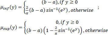
Equations [1.2] and [1.3] show that:
Notice that if ymin ≤ min{f(x): x ∈ Ω} and ymax ≥ max {f(x): x ∈ Ω}, then μinf(y1) = 0, while μinf(ym+1) = b − a and we have:
Let
Then,
and
Thus,
where the integral in this formula is a Riemann one. So,
Analogously,
so that
Thus, we have
and
Equations [1.5] and [1.6] show that:
Notice that, if ymin ≤ min{f(x): x ∈ Ω} and ymax ≥ max{f(x): x ∈ Ω}, then μsup(y1) = b − a, while μsup(yM+1) = 0 and we have:
1.3. Matlab® classes for a Riemann integral by trapezoidal integration
The one-dimensional (1D) trapezoidal rule is implemented in Matlab® in the intrinsic function trapz and may be extended to multidimensional situations. Assume that the structure p has fields p.x, p.y, p.z corresponding to the coordinates of the points xi, yj, zk of the partitions of the intervals and p.dim corresponding to the dimension, while table F contains the values of ƒ - Fi = ƒ(xi), or Fij = ƒ(xi, yj) or Fijk = ƒ(xi, yj, zk), according to the dimension of the integral. Let us summarize the data in a structure data such that data.points = p and data.values = F. Then we may use the class below (Program 1.1).


Program 1.1. A class for the evaluation of Riemann integrals
This class contains only trapezoidal and mean value integration methods, but it can be enriched by the user with other methods of numerical integration.
EXAMPLE 1.1.– Let us evaluate:
by using the points x=0:0.01:1; and y=0:0.01:2;. Assuming that F(i,j)=x(i)^2+y(j)^2;, the code:
p.x = x;
p.y = y;
p.dim = 2;
p.measure = 2;
data.points = p;
data.values = F;
v1 = riemann.trpzd(data)
v2 = riemann.mean_value(data)
produces v1 = 3.3334, v2 = 3.3433. The exact value is ![]() .
.
![]()
EXAMPLE 1.2.– Let us evaluate:
by using the points x=0:0.01:1;,y=0:0.01:2;, z=0:0. 01:3. Assuming that F(i,j,k)=x(i)^2+y(j)^2+z(k)^2, the code:
p.x = x;
p.y = y;
p.z = z;
p.dim = 3;
p.measure = 6;
data.points = p;
data.values = F3;
v1 = riemann.trpzd(F3,p)
v2 = riemann.mean_value(F3,p)
produces v1 = 28.0003, v2 = 28.0600. The exact value is 28.
![]()
The creation of the tables F from a subprogram f evaluating a function ƒ is made by the following class:


This class generates a table of values Fi = ƒ(xi), Fij = F(xi, yj), Fij = F(xij,yij), Fijk = ƒ(xi, yj, zk), or Fijk = ƒ(xijk, yijj, zijk), according to the data furnished. Data is stored in the structure p: p.dim is the dimension, p.x, p.y, p.z are the coordinates. Method takes the value “vector” or “array” according to the dimensions of p.x, p.y, p.z. For instance, the code:
x = 0:0.1:1;
y = 0:0.1:2;
f = @(x) sum(x.^2);
p.x = x;
p.y = y;
p.dim = 2;
[X,Y] = meshgrid(x,y);
xx = permute(X,[2 1]);
yy = permute(Y,[2 1]);
F1 = spam.partition(f,p);
F2 = spam.points('table',f,xx,yy);
v = sqrt(sum(sum((F1-F2).^2)));
produces as result v=0. Both the tables F1 and F2 coincide, but F1 is generated by using vectors x and y, while F2 is generated using two-dimensional (2D) arrays. Adding the lines:
z = 0:0.1:3;
p.z = z;
p.dim = 3;
[X,Y,Z] = meshgrid(x,y,z);
xx = permute(X,[2 1 3]);
yy = permute(Y,[2 1 3]);
zz = permute(Z,[2 1 3]);
F1 = spam.partition(f,p);
F2 = spam.points('table',f,xx,yy,zz);
v3 = sqrt(sum(sum(sum((F1-F2).^2))));
produces as result v3=0: the resulting arrays are equal. Here, F1 is generated by using vectors x, y and z, while F2 is generated using three-dimensional (3D) arrays.
Notice that the class Riemann requests data in the vector form. The extension to data defined in the array form will be useful for integration using the intrinsic functions of Matlab (see section 1.6).
1.4. Matlab® classes for Lebesgue’s integral
Equations [1.4] and [1.7] provide a practical method for the evaluation of I: the Lebesgue integral is replaced by a Riemann one, which may be numerically evaluated by quadrature methods using the values μinf(y1), ... , μinf(yM+1) (when using equation [1.4]) or μsup(y1), ... , μsup(yM+1) (when using equation [1.7]). The construction of the values of μinf or μsup is performed by using the subdivision of Ω: for each i, the measure of the part of Ωi belonging to Ѕinf(y) (respectively, Ѕsup(y)) is estimated and added to μinf(yi) (respectively, μSup(yi)) For instance, we may use the following class:


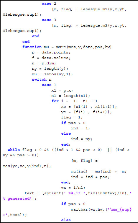


Program 1.3. A class for the evaluation of Lebesgue integrals
At a glance, we see that this class is more complex than the class Riemann. This is due to the fact that two partitions are requested and must be treated. Methods inf_el and sup_el determine the part of (xj−1, xj), 1 ≤ j ≤ N, which belongs to Ѕinf(yi) and Ѕsup(yi), respectively. These subprograms return approximations of the Lebesgue measure of the part of (x1, x2) lying in the region of interest (Ѕinf(yt) for mes_inf or Ѕsup(yt) for mes_sup). The special cases where either y1 = –∞ or y2 = +∞ are treated by considering that a half of the interval (x1, x2) belongs to the region of interest – this choice is arbitrary and may be modified by the user. For the standard situation where both y1 and y2 are real numbers, a linear interpolation determines the part of the interval belonging to the region of interest – this choice may also be modified by the user. When using this class, the evaluation of the integral involves the choices, on the one hand, the choice of the evaluation points (vector y) and, on the other hand, the choice among the use of μinf (equation [1.4]), of μsup (equation [1.7]) or the arithmetic mean of these results. In addition, it is possible to reduce the time of computation by evaluating these measures in a limited number of points and using the interpolation function interp1 for the evaluation of the integral. The functions μinf, μsup are evaluated, respectively, by the methods measure inf and measure_sup, both returning a function generated by interpolation of the evaluated values, using interp1 and the interpolation method interpmet.
EXAMPLE 1.3.– Let us consider Ω = (−1,1) and ƒ(x) = x2. Then,

For N = 1024, M = 128, ymin = −0.5, ymax = 1.5, a = −1, b = 1, the code:
hx = (b-a)/N;
x = a + hx*(0:N);
f = x.^2;
p.x = x;
p.dim = 1;
data.points = p;
data.values = f;
mu1 = lebesgue.measure_inf(y,data,'linear');
mu2 = lebesgue.measure_sup(y,data,'linear');
furnishes

Figure 1.4. Lebesgue measure obtained in example 1.3
The code:
I1 = lebesgue.integrate(y,data,'inferior','linear');
I2 = lebesgue.integrate(y,data,'superior','linear');
I3 = lebesgue.integrate(y,data,'mean','linear')
furnishes I1 = 0.66746, I2 = 0.66746 and I3 = 0.66746. The exact value is 2/3 ≈ 0.66667. These results may be improved by refining the partitions, namely on the vertical axis. For instance, N = 4096, M = 512 lead to I1 = 0.66677, I2 = 0.66677 and I3 = 0.66677.
![]()
When regular functions are considered – this is the case in example 1.3 – Lebesgue’s approach is not the more efficient one. For instance, Riemann’s approach furnishes more precise results. However, for functions having discontinuity points, Lebesgue’s approach may be interesting (see examples below).
EXAMPLE 1.4.– Let us consider Ω = (0,2) and ![]() . Then,
. Then,
Using M = 256, ymin = 0, ymax = 100, N = 4096, we obtain I1 = 2.7905, I2 = 2.7906, I3 = 2.7906, while the trapezoidal rule trapz(x,f) returns the value Inf. The exact value is 2*sqrt(2) ≈ 2.8284. For M = 1024, N = 4096, we have I1 = I2 = I3 = 2.7959 and trapz (x,f) returns the value Inf. The measures μinf and μsup are in Figure 1.5.
![]()

Figure 1.5. Results for example 1.4
EXAMPLE 1.5.– Let us consider Ω = (0,20) and ƒ(x) = log(|sin(πx)|). Then,
In this case, when using N = 1024, ymin = −2.5, ymax = 0.5, M = 256, we obtain I1 = I2 = I3 =−10.121, while trapz(x,f) returns the value-Inf. For N = 4096, ymin = −100, ymax = 0.5, M = 1024, the values are I1 = −14.3736, I2 = −14.3733, I3 = −14.3735 and trapz(x,f) returns the value-Inf. The measures μinf and μsup are in Figure 1.6.
![]()

Figure 1.6. Lebesgue measure in example 1.5
EXAMPLE 1.6.– Let us consider Ω = (0,20) and ƒ(x) = sign(sin(πx)). Then,
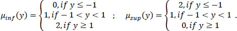
In this case, using N = 1024, ymin = −1.5, ymax = 1.5, M = 256, we obtain I1= I2 = I3 =0.0097659 and trapz(x,f) returns the value 0.0098. The exact value is 0. The measures μinf and μsup are given in Figure 1.7.
![]()

Figure 1.7. Results for Lebesgue measure in example 1.6
One of the interesting features of Lebesgue integrals is the fact that multidimensional integration reduces to 1D integration: indeed, only the evaluation of μinf, μsup involves multidimensional calculations.
Once these quantities are obtained, equation [1.4] or equation [1.7] is used in order to evaluate the integral – only 1D integration is involved in this calculation. Examples are given below.
EXAMPLE 1.7.– Let us evaluate:
by using the points x=0:step:1; and y=0:step:2; with step = 0.01. Assuming that F(i,j)=x(i)^2+y(j)^2, the code:
p.x = x;
p.y = y;
p.dim = 2;
yleb = 0:0.1:5;
data.points = p;
data.values = F;
I1 = lebesgue.integrate(yleb,data,'inferior','linear');
I2 = lebesgue.integrate(yleb,data,'superior','linear');
I3 = lebesgue.integrate(yleb,data,'mean','linear')
produces I1=I2=I3=3.3334. The exact value is ![]() .
.
![]()
EXAMPLE 1.8.– Let us evaluate:
by using the points x=0:step: 1; ,y=0 :step:2;, z=0: step: 3;, with step = 0.05. Assuming that F(i,j,k)=x(i) ^2+y(j)^2 +z(k) ^2, the code:
p.x = x;
p.y = y;
p.z = z;
p.dim = 3;
yleb = 0:0.2:14;
data.points = p;
data.values = F;
I1 = lebesgue.integrate(yleb,data,'inferior','linear');
I2 = lebesgue.integrate(yleb,data,'superior','linear');
I3 = lebesgue.integrate(yleb,data,'mean','linear')
produces I1=I2=I3=28.0094.
Using as interpolation method ‘cubic’ (or ‘pchip’, for newer versions of Matlab®) produces the result 28.0090. The exact value is 28.
![]()
1.5. Matlab® classes for evaluation of the integrals when ƒ is defined by a subprogram
Let us assume that the values of ƒ(x) are furnished by a subprogram f.m which receives as argument a vector x and returns a value f (x).
The internal functions for numerical integration are given in Table 1.1. Notice that ay,by,az, bz are function handles, i.e. anonymous functions or subprograms evaluating functions.
In order to use these intrinsic functions of Matlab®, we must transform f. Indeed, the intrinsic functions of Matlab® assume as arguments (x,y) or (x,y,z) and not a vector x. Moreover, they assume that the functions may receive multidimensional arrays of data and return a corresponding array of results. The adaptation is made by the subprograms of class spam. For instance, we may use the class given in program 1.4.
Table 1.1. Intrinsic functions for the evaluation of integrals


Program 1.4. A class for the integration of functions defined by subprograms
In this program, limits (or xlim) is a data structure with the properties dim, lower, upper, which define dimension, lower and upper bounds for the integral, respectively.
EXAMPLE 1.9.– Let us consider the integration of:
In this case,

This program produces v = 0.2358. The exact value is ![]() .
.
![]()
EXAMPLE 1.10.– Let us consider the evaluation of the volume of a sphere. The code:

produces the result v = 4.1888. The exact result is ![]() . But the code:
. But the code:

Program 1.7. Evaluation of a 3d integral with a discontinuous function
produces an unsuccessful run: the result is v = NaN.
![]()
The intrinsic functions for older versions of Matlab® are given in Table 1.2. triplequad adapts to the same use as integral3 by considering a box containing the region of integration and extending the integrand by zero outside the region of integration.
Notice that both dblquad and triplequad assume that ƒ accepts as input a vector x and scalars y and z and returns a vector of results, so that the preceding functions spam2 and spam3 have to be modified in order to satisfy these requirements.
Table 1.2. Intrinsic function for older versions of Matlab®0

1.6. Matlab® classes for partitions including the evaluation of the integrals
Partitions may be assimilated to finite element meshes. For instance, in Matlab®, we may define classes having convenient properties and methods. For the situation where Ω = (a, b) ⊂ ![]() , an example of such a class is given in program 1.8. Notice that the class includes a method for integration (it assumes finite values for all the elements of F).
, an example of such a class is given in program 1.8. Notice that the class includes a method for integration (it assumes finite values for all the elements of F).
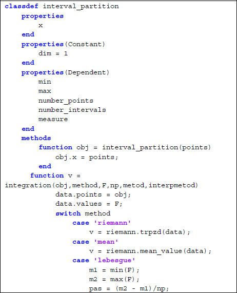

Program 1.8. Definition of a class for partition of intervals
For instance, the code:
pas = 0.05;
x = 0:pas:1;
p = interval_partition(x);
creates the structure p of type interval_partition. Then,
f = @(x) exp(x);
F = spam.mapspam('vector',f,x);
v1 = p.integration('riemann',F)
v2 = p.integration('lebesgue',F,20,'inferior','pchip')
v3 = p.integration('mean',F)
evaluates the integral ![]() using the trapezoidal rule or Lebesgue’s method with 20 intervals on the vertical axis. For the points given, the result is v1 = 1.7186, v2 = 1.7187, v3=1.7253. It may be improved by considering a partition containing a larger number of points. For instance, if pas = 0.01; the result is v1 = v2 = 1.7183, v3 = 1.7197.
using the trapezoidal rule or Lebesgue’s method with 20 intervals on the vertical axis. For the points given, the result is v1 = 1.7186, v2 = 1.7187, v3=1.7253. It may be improved by considering a partition containing a larger number of points. For instance, if pas = 0.01; the result is v1 = v2 = 1.7183, v3 = 1.7197.
For Ω = (a1, b1) × (a2, b2) we may define a class as follows:


For instance, the code:
pas = 0.05;
x = 0:pas:1;
y = 0:pas:2;
pp = rectangular_partition(x,y);
creates the structure pp of type rectangular_partition and the code:
f = @(x) exp(x(1) - x(2));
F = spam.mapspam('vector',f,pp);
v1 = pp.integration('trapezoid',F);
v2 = pp.integration('tri13',F);
v3 = pp.integration('tri24',F);
v4 = pp.integration('quad',F);
v5= pp.integration('lebesgue',F,40,'inferior','pchip');
v6= pp.integration('lebesgue',F,40,'superior','pchip');
v7 = pp.integration('lebesgue',F,40,'mean','pchip');
produces v1 = v4 = 1.4864, v2 = 1.4860, v3 = 1.4867, v5 = v6 = v7 = 1.4861. The exact value is (e − 1)(1 − e−2) ≈ 1.4857. When using pas = 0.01, the result is v1 = v2 = v3 = v4 = 1.4858, v5=v6=v7=1.4856.
EXAMPLE 1.11.– Let us consider the integration of ƒ(x) = x1e−x2 on Ω = (0,1) × (0,2). The exact value of the integral is ![]() . Using pas = 0.05, the results are v1=v2=v4=v5=3.1946, v2=0.8597, v6=3.1942. For pas=0.01, v1=v2=v4=v5=3.1946, v3=3.1945, v6=3.1942, v7=3.1944.
. Using pas = 0.05, the results are v1=v2=v4=v5=3.1946, v2=0.8597, v6=3.1942. For pas=0.01, v1=v2=v4=v5=3.1946, v3=3.1945, v6=3.1942, v7=3.1944.
![]()
EXAMPLE 1.12.– Let us consider the integration of
on Ω = (0,1) × (0,1). This situation corresponds to the integration of
and the exact value of the integral is ![]() . Using pas = 0.01 and np=100 intervals on the vertical axis, the results are v1=v2=v4=0.2344, v3=0.2345, v5 = 0.2363, v6 = 0.2344, v7 = 0.2354. Due to discontinuity, finer partitions are requested for a good precision.
. Using pas = 0.01 and np=100 intervals on the vertical axis, the results are v1=v2=v4=0.2344, v3=0.2345, v5 = 0.2363, v6 = 0.2344, v7 = 0.2354. Due to discontinuity, finer partitions are requested for a good precision.
![]()
In 3D situations, Ω = (a1, b1) × (a2, b2) × (a3, b3), we may define a class containing methods for integration by trapezoidal rule or integration using a tetrahedral or hexahedral mesh as follows:


For instance, the code:
pas = 0.05;
x = 0:pas:1;
y = 0:pas:2;
z = 0:pas:3;
ppp = cobble_partition(x,y,z);
creates the structure pp of type cobble partition. The code:
v1 = ppp.integration('trapezoid',F);
v2 = ppp.integration('tetra5',F);
v3 = ppp.integration('tetra6',F);
v4 = ppp.integration('hexa',F);
v5=ppp.integration('lebesgue',F,40,'inferior','pchip');
v6=ppp.integration('lebesgue',F,40,'superior','pchip');
v7=ppp.integration('lebesgue',F,40,'mean','pchip');
produces v1 = v4 = 13.3791, v2 = 13.3789, v3 = 13.3763, v4 = 13.3791, v5 = 13.4117, v6 =13.4086, v7 = 13.4102. The exact value is 9(e − 1)(1 − e−2) ≈ 13.3716.
EXAMPLE 1.13.– Let us consider the evaluation of the 3D integral:
We may consider Ω = (−1,1) × (−1,1) × (−1,1) and
Then, we evaluate:
Using pas = 0.05, the result obtained is v1 = v2 = v3 = v4 = 4.1714, v5 = v6 = v7 = 4 . 1724. The exact result is ![]() .
.
![]()
REMARK.– In some situations, the available data is not on a grid, but just on sparse points. This situation is considered in Chapter 3.
![]()