
4
Functional Spaces for Engineers
Functional spaces are Hilbert spaces formed by functions. For engineers, these spaces represent spaces of quantities having a spatial or temporal distribution, i.e. fields. For instance, the field of temperatures on a region of the space, the field of velocities of a continuous medium, the history of the velocities of a particle is functions. As previously observed, these spaces have some particularities connected to the fact that they are infinite dimensional.
From the beginning of the 20th Century, the works of Richard Courant, David Hilbert, Kurt Friedrichs and other mathematicians of Gottingen have pointed the necessity of a redefinition of derivatives and of the functional spaces involving derivatives.
Otto Nykodim introduced a class named “BL” (class of Bepo-Levi), involving (u, v) = ∫∇u.∇v dx [NIK 33]. He constructed a theory about this class and brought it to the framework of Hilbert spaces two years later [NIK 35], but the complete theory arrived later with the works of Serguei Sobolev, a Russian mathematician that introduced functional spaces fitting to variational methods.
Sobolev was closely connected to Jacques Hadamard, who faced the mathematical difficulties arising in fluid mechanics, when studying the Navier–Stokes equations [HAD 03a, HAD 03b]. Far from Hadamard, the Russian Nikolai Gunther, a former PhD student of Andrey Markov, was interested in potential theory and, particularly, in extensions of Kirchhoff formula and derivatives of irregular functions by a new smoothing method. Gunther suggested, in collaboration with Vladimir Smirnov, a promising PhD student – Serguei Sobolev. Hadamard was a frequent visitor of Sobolev and was in contact with him since 1930. At these times, Sobolev was working at the Seismological Institute of the Academy of Sciences in Leningrad (now Saint Petersburg), under the direction of Smirnov, and studied the propagation of waves in inhomogeneous media [SOB 30, SOB 31]. During this work, he formulated a method of generalized solutions [SOB 34a, SOB 34b, SOB 35a, SOB 35b], which was rapidly diffused in France by Jacques Hadamard and Jean Leray. This last mathematician then applied the nascent – and imperfect – theory to fluid mechanics and obtained a fundamental result, by using a new notion of derivative [LER 34].
World War II interrupted the advances of variational methods, notably in the works of Laurent Schwartz and Israel Gelfand, who popularized the works of Sobolev among mathematicians and developed the extension of their applications considerably. The end of the war was to produce their more interesting works. For instance, the fundamental work of Schwartz appeared in 1945 [SCH 45] and the complete theory was published in 1950–1951 [SCH 50, SCH 51]. Gelfand published his major works in 1958–1962 [GEL 64a, GEL 68b, GEL 63c, GEL 64b, GEL 66]. The works of Schwarz and Gelfand diffused the new theory worldwide and led to fantastic developments in terms of solution of differential equations – we will study this aspect in the next chapter.
These works did not signal the end in the development of functional spaces connected to variational methods. Namely, the works of Jean-François Colombeau [COL 84] led to a response to the objections of Schwarz in [SCH 54] and the theory of hyper functions generalized his works [SAT 59a, SAT 60]. These new developments still need to find engineering applications and will thus not be studied in this book.
4.1. The L2(Ω) space
The construction of complete function spaces is complex: as shown in the preceding examples, there is a contradiction between the assumptions of regularity used in order to verify that (u, u) = 0 ⇒ u = 0 and the assumption that Cauchy sequences have a limit in the space.
Such a difficulty has been illustrated, for instance, in example 3.5, with ![]() is continuous on Ω and (v, v) < ∞} and
is continuous on Ω and (v, v) < ∞} and
In this example, we have shown a sequence {un: n ![]()
![]() *} such that un → u strongly, but
*} such that un → u strongly, but ![]() . In order to overcome this difficulty, the method of completion has been introduced. Completion consists of generating a new vector space, referred to as L2 (Ω) and formed by sets of Cauchy sequences on V (see [SOU 10]). L2(Ω) may be interpreted as follows: let V be the set of continuous square summable functions:
. In order to overcome this difficulty, the method of completion has been introduced. Completion consists of generating a new vector space, referred to as L2 (Ω) and formed by sets of Cauchy sequences on V (see [SOU 10]). L2(Ω) may be interpreted as follows: let V be the set of continuous square summable functions:
and
Then
is a Hilbert space (see [SOU 10]). Indeed, in this case,
In general, in order to alleviate the notation, the square brackets are not written and [v] is denoted by v. When using this simple notation, we must keep in mind that v (i.e. [v]) contains infinitely many elements, so that u(x) has no meaning. For instance, let us consider,
Then, ∀α ![]()
![]() ,uα
,uα ![]() [0]. So, [uα] = [0] and, uα(x) = α, so that the class of the null function contains an infinite amount of elements and the value of
[0]. So, [uα] = [0] and, uα(x) = α, so that the class of the null function contains an infinite amount of elements and the value of ![]() has no meaning. When denoting [0] by 0, we must keep in mind that the values of 0 in a particular point vary. By these reasons, elements of L2(Ω) are sometimes referred to as generalized functions and completion implies a loss of information: point values are lost when passing to the complete space L2(Ω). In order to help the reader to keep in mind the difference between u and [u], we will use the notation:
has no meaning. When denoting [0] by 0, we must keep in mind that the values of 0 in a particular point vary. By these reasons, elements of L2(Ω) are sometimes referred to as generalized functions and completion implies a loss of information: point values are lost when passing to the complete space L2(Ω). In order to help the reader to keep in mind the difference between u and [u], we will use the notation:
Thus, index zero recalls that the elements on the scalar products are not standard functions, but classes, for which point values are not defined.
It must be noted that the construction of L2(Ω) may be carried using other spaces ![]() such as, for instance,
such as, for instance,

or
![]() is often referred to as the set of test functions. A square summable function may be approximated by elements of these spaces, namely by using mollifiers introduced by Sobolev [SOB 38] and Friedrichs [FRI 44, FRI 53]. Moreover, these spaces are dense in L2(Ω).
is often referred to as the set of test functions. A square summable function may be approximated by elements of these spaces, namely by using mollifiers introduced by Sobolev [SOB 38] and Friedrichs [FRI 44, FRI 53]. Moreover, these spaces are dense in L2(Ω).
In the following, this approach is generalized by Sobolev spaces, and a way to retrieve the notion of point values is given.
4.2. Weak derivatives
As observed above, passing from standard functions to generalized functions involves the loss of the notion of point values. This implies that the standard notion of derivative does not apply. Indeed, let Ω = (a,b), v ![]() L2(Ω): the quotient used to define the derivative at point x
L2(Ω): the quotient used to define the derivative at point x ![]() Ω reads as
Ω reads as ![]() and has no meaning, since the values of v(x) and v(x + h) are undefined. Distribution theory proposed by Schwarz introduces a new concept, based on the integration by parts. Indeed, assume that v:Ω →
and has no meaning, since the values of v(x) and v(x + h) are undefined. Distribution theory proposed by Schwarz introduces a new concept, based on the integration by parts. Indeed, assume that v:Ω → ![]() is regular enough.
is regular enough.
and, for a regular function φ such that φ(a) = φ(b) = 0,
so that v′ is characterized by the linear functional
This remark suggests the following definition:
DEFINITION 4.1.– Let Ω ⊂ ![]() n be a regular domain and u
n be a regular domain and u ![]() L2(Ω). The weak derivative
L2(Ω). The weak derivative ![]() is the linear functional
is the linear functional ![]() defined by:
defined by:
![]()
Weak derivatives are also referred to as distributional derivatives or generalized derivatives. We have:
THEOREM 4.1.– Let ![]() be the weak derivative ∂u/∂xi, and verify:
be the weak derivative ∂u/∂xi, and verify:
Then, there exists a unique wi ![]() L2 (Ω) such that,
L2 (Ω) such that,
In this case, we say that wi = ∂u/∂xi.
![]()
PROOF–. Theorem 3.23 shows that ℓi extends to a linear continuous functional ℓi:L2(Ω) → ![]() . Therefore, the result is a consequence of Riesz (theorem 3.24).
. Therefore, the result is a consequence of Riesz (theorem 3.24).
![]()
COROLLARY 4.1.– Let ψ ![]() C1(Ω)be such that both ψ and ∇ψ are square summable. Let u = [ψ]
C1(Ω)be such that both ψ and ∇ψ are square summable. Let u = [ψ] ![]() L2(Ω). Then ∂u/∂xi = ∂ψ/∂xi, for 1 ≤ i ≤ n, i.e. the weak and classical derivatives coincide.
L2(Ω). Then ∂u/∂xi = ∂ψ/∂xi, for 1 ≤ i ≤ n, i.e. the weak and classical derivatives coincide.
![]()
PROOF.– We observe that:
Thus, Green’s formula:
yields:
so that, taking M = ||∂ψ/∂xi||0,
and the result follows from theorem 4.1.
![]()
REMARK 4.1.– Standard derivation rules apply to weak derivatives, under the assumption that each element is defined. For instance, if ![]() , then,
, then,
However, in derivatives of composite functions, change of variables have the same properties as classical derivatives, provided each element is defined.
![]()
EXAMPLE 4.1.– Let Ω = (−1, 1), u(x) = |x|. Let us show that u’(x) = sign(x). Indeed,
and we have (recall that φ(−1) = φ(1) = 0).

Thus,
![]()
EXAMPLE 4.2.– Let Ω = (−1, 1), u(x) = sign(x). Let us show that u’ = 2δ0, with δ0(φ) = φ(0) [Dirac’s delta – see Chapter 6]. Indeed,
and we have (recall that φ(−1) = φ(1) = 0).
In this case, there is no w ![]() L2(Ω) such that ℓ(v) = (w, v)0, ∀v
L2(Ω) such that ℓ(v) = (w, v)0, ∀v ![]() L2(Ω).
L2(Ω).
![]()
4.2.1. Second-order weak derivatives
We have, for Ω = (a,b), ![]() (thus, φ(a) = φ(b) = φ′(a) = φ′(b) = 0)
(thus, φ(a) = φ(b) = φ′(a) = φ′(b) = 0)
Then, we may define:
DEFINITION 4.2.– Let Ω ⊂ ![]() n be a regular domain and u
n be a regular domain and u ![]() L2(Ω). The weak derivative ∂2u/∂xi ∂xj is the linear functional
L2(Ω). The weak derivative ∂2u/∂xi ∂xj is the linear functional ![]() defined by:
defined by:
![]()
Analogous to theorem 4.1, we have:
THEOREM 4.2.– Let ![]() be the weak derivative ∂2u/∂xi ∂xj, and verify:
be the weak derivative ∂2u/∂xi ∂xj, and verify:
Then, there exists a unique wij ![]() L2 (Ω) such that:
L2 (Ω) such that:
![]()
In this case, we say that wij = ∂2u/∂xi ∂xj.
The proof is analogous to these given in theorem 4.1.
EXAMPLE 4.3.– Let Ω = (−1, 1), u(x) = |x|. Let us show that u" = 2δ0, with δ0(φ) = φ(0) (Dirac’s delta, see Chapter 6). Indeed,
and we have (recall that φ′(−1) = φ′(1) = 0):
![]()
4.2.2. Gradient, divergence, Laplacian
Let Ω ⊂ ![]() n be a regular domain. Let u
n be a regular domain. Let u ![]() L2(Ω). The gradient of u, denoted by ∇u, is defined as
L2(Ω). The gradient of u, denoted by ∇u, is defined as ![]() , given by:
, given by:

The Laplacian of u, denoted by Δu, is defined as ![]() , given by:
, given by:
Let u = (u1, …, un) ![]() [L2(Ω)]n. The divergence of u, denoted by div(u), is defined as
[L2(Ω)]n. The divergence of u, denoted by div(u), is defined as ![]() , given by:
, given by:
REMARK 4.2.– Classical results such as Green’s formulas or Stokes’ formula remain valid when using weak derivatives, under the assumption of each term has a meaning. For instance,
under the condition that each term (including products) is defined.
![]()
EXAMPLE 4.4.– Let ![]() , u(x) = ln r,
, u(x) = ln r, ![]() . Let us show that Δu = 2πδ0. Let
. Let us show that Δu = 2πδ0. Let ![]() ,
, ![]() . Notice that
. Notice that ![]() , so that the weak and classical derivatives coincide on Ωε. Then, Green’s formula shows that:
, so that the weak and classical derivatives coincide on Ωε. Then, Green’s formula shows that:
Since ![]() on ∂Ω,
on ∂Ω,
Using polar coordinates (r, θ) and taking into account that ![]() ,
, ![]() ds = rdθ and that r = εon ∂Ωε, we have:
ds = rdθ and that r = εon ∂Ωε, we have:
Since ε ln ε → 0 and
we have:
Thus,
![]()
EXAMPLE 4.5.– Let ![]() ,
, ![]() ,
, ![]() . Analogously to the preceding situation, we have
. Analogously to the preceding situation, we have ![]() . In this case,
. In this case, ![]() ,
, ![]() and, using spherical coordinates (r, θ, ψ), we have
and, using spherical coordinates (r, θ, ψ), we have ![]() ds = r2 sinψdθdψ and that r = ε on ∂Ωε, so that
ds = r2 sinψdθdψ and that r = ε on ∂Ωε, so that
Thus
and
![]()
4.2.3. Higher-order weak derivatives
We have, for Ω = (a, b), φ ∈ ![]() (Ω),
(Ω),
Thus, we may define:
DEFINITION 4.3.– Let Ω ⊂ ![]() n be a regular domain and v ∈ L2(Ω). Let
n be a regular domain and v ∈ L2(Ω). Let ![]() . The weak derivative
. The weak derivative ![]() is the linear functional
is the linear functional ![]() defined by:
defined by:
![]()
We have:
THEOREM 4.3.– Let ![]() be the weak derivative
be the weak derivative ![]() and verify:
and verify:
Then, there exists a unique wα ∈ L2(Ω) such that:
In this case, we say that ![]()
![]()
The proof is analogous to those given in theorem 4.1.
4.2.4. Matlab® determination of weak derivatives
Approximations of classical derivatives may be obtained by using the method derive defined in the class basis introduced in section 2.2.6. The evaluation of weak derivatives requests the use of scalar products, analogous to those defined in section 3.2.5. We present below a Matlab implementation using this last class. Recall that du = u′ verifies:
Let us consider a basis {φi:i ∈ ![]() } ⊂ S and
} ⊂ S and
We have:
Thus, vector DU = (du1, … , dun) is the solution of a linear system A. DU = B, where ![]() .
.
Let us assume that the family ![]() is defined by a cell array basis such that basis{i} defines φi according to the standard defined in section 3.2.6: basis{i} is a structure having properties dim, dimx, component, where component is a cell array such that each element is a structure having as properties value and grad. u is assumed to be analogously defined. In this case, the weak derivative is evaluated as follows (Program 4.1):
is defined by a cell array basis such that basis{i} defines φi according to the standard defined in section 3.2.6: basis{i} is a structure having properties dim, dimx, component, where component is a cell array such that each element is a structure having as properties value and grad. u is assumed to be analogously defined. In this case, the weak derivative is evaluated as follows (Program 4.1):


Program 4.1. A class for weak derivatives of functions of one variable
EXAMPLE 4.6.– Let us consider the family φi(x) = xi−1 and u(x) = x4 The weak derivative is u′(x) = 4x3. We consider a = −1, b = 1. We generate the function by using the commands:
xlim.lower.x = a;
xlim.upper.x = b;
xlim.dim = 1;
u.dim = 1;
u.dimx = 1;
u.component = cell(u.dim,1);
u.component{1}.value = @(x) x^4;
ua = u.component{1}.value(a);
ub = u.component{1}.value(b);
Then, the commands
sp_space = @(u,v) scalar_product.sp0(u,v,xlim,'subprogram');
c = weak_derivative.coeffs(u,basis,sp_space,a,b,ua,ub,'subprogram');
du = weak_derivative.funcwd(c,basis);
generate the weak derivative by using the method “subprogram”. We may also generate a table containing the values of u as follows:
x = a:0.01:b;
p.x = x;
p.dim = 1;
U.dim = 1;
U.dimx = 1;
U.component = cell(U.dim,1);
U.component{1}.value = spam.partition(u.component{1}.value,p);
The commands
sp_space = @(u,v) scalar_product.sp0(u,v,p,'table');
ctab = weak_derivative.coeffs(U,tb,sp_space,a,b,ua,ub,'table');
dutab = weak_derivative.funcwd(ctab,basis);
generate the weak derivative by using the method “table”. The results are shown in Figure 4.1.
![]()
EXAMPLE 4.7.– Let us consider the family ![]() and u(x) = |x|. The weak derivative is u′(x) = sign(x). We consider a = −1, b = 1. The results are exhibited in Figure 4.2.
and u(x) = |x|. The weak derivative is u′(x) = sign(x). We consider a = −1, b = 1. The results are exhibited in Figure 4.2.
![]()

Figure 4.1. Evaluation of the weak derivative of x4 using subprograms and tables
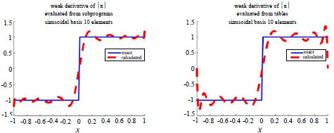
Figure 4.2. Evaluation of the weak derivative of |x| using subprograms and tables
4.3. Sobolev spaces
As previously indicated, Serguei Lvovitch Sobolev was the Russian mathematician that introduced functional spaces fitting to variational methods, giving a complete mathematical framework. In his works, Sobolev formulated a theory of variational solutions and introduced Hilbert spaces involving derivatives [SOB 64], such as, for instance,
and

We may also consider Γ ⊂ ∂Ω such that meas(Γ) ≠ 0, i.e. Γ has a strictly positive length if its dimension is 1 and a strictly positive surface if its dimension is 2:

Sobolev spaces are generated by completion of particular spaces [SOB : 8]. For instance, by considering
![]() and∇v are continuous on Ω and (v, v)1<∞}
and∇v are continuous on Ω and (v, v)1<∞}
with the scalar product
the completion method generates H1(Ω). Analogously, the completion
generates ![]() . Taking Γ = ∂Ω. generates
. Taking Γ = ∂Ω. generates ![]() .
.
The generic Sobolev space is denoted by:
and has a scalar product:
It is obtained by completion of a convenient space of continuous functions. We have H0(Ω) = L2(Ω).
Sobolev spaces are often invoked when solving partial differential equations. Note that they are formed by generalized functions.
One of the main properties of elements of Sobolev spaces are inequalities connecting an element and its weak derivatives. These inequalities are often referred to as Sobolev imbedding inequalities. For instance, we have Morrey’s inequality (see [EVA 10]).
THEOREM 4.4.– There exists ![]() ∈
∈ ![]() such that
such that
![]()
and Poincaré’s inequality (see [EVA 10]).
THEOREM 4.5.– Let Ω ⊂ ![]() n be open bounded, not empty. There exists
n be open bounded, not empty. There exists ![]() ⊂
⊂ ![]() such that:
such that:
![]()
Sobolev spaces are separable (see, for instance, [LEB 96]).
4.3.1. Point values
The point value may have a meaning for elements from Sobolev spaces other than H0(Ω). For instance, let us consider Ω = (a,b) and u ∈ H1(Ω)We have:
Let λ ![]()
![]()
We have:
so that,
This equality may be used to determine u(b). Let us define:
and ℓb:![]() →
→![]() given by:
given by:
Tb is linear, so that ℓb is also linear. We have:
Moreover, there exists C ![]()
![]() such that,
such that,
Then, ℓb:![]() →
→![]() is linear and continuous. From the Riesz theorem, there exists β
is linear and continuous. From the Riesz theorem, there exists β ![]()
![]() such that ℓb (λ) = βλ. We define u(b) =β
such that ℓb (λ) = βλ. We define u(b) =β
The map H1(Ω) ∋ u → β ![]()
![]() is the trace of u at b., denoted by γu.
is the trace of u at b., denoted by γu.
It generalizes to higher dimension by considering Ω ⊂ ![]() n, u
n, u ![]() H1(Ω), Γ ⊂ ∂Ω – in this case, we use the Green’s formula:
H1(Ω), Γ ⊂ ∂Ω – in this case, we use the Green’s formula:
We may consider, for instance, ƒ ![]() L2(Γ) and
L2(Γ) and
In this case,
and this equality may be used in order to define u on Γ, into an analogous way. Here,
Again, TΓ is linear and
so that the existence of C ![]()
![]() such that:
such that:
yields that ℓΓ: L2(Γ) → ![]() is linear and continuous. In this case, from the Riesz theorem, there exists g
is linear and continuous. In this case, from the Riesz theorem, there exists g ![]() L2 (Γ) such that,
L2 (Γ) such that,
We define γu = g on Γ.
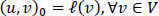
4.4. Variational equations involving elements of a functional space
Variational equations were introduced in Chapter 3 when considering orthogonal projections (equations [3.5], [3.7], [3.8]) and in Chapter 2.
The standard form of a variational equation is:
where H ⊂ V is a linear subspace, ℓ: V → ![]() is linear continuous and
is linear continuous and ![]() is such that v → a(u, v) is linear. The standard formulation includes situations where the variational equation is a nonlinear one. For orthogonal projections, only linear or affine situations have to be considered:
is such that v → a(u, v) is linear. The standard formulation includes situations where the variational equation is a nonlinear one. For orthogonal projections, only linear or affine situations have to be considered:
- 1) In the case of the orthogonal projection Px of x
 V onto a vector subspace H, u = Px H, a(u, v) is the scalar product (u, v), ℓ(v) = (x, v) and H = S.
 - 2) In the case of the orthogonal projection Px of x V onto an affine subspace S = S0 + {x0} (S0 vector subspace, x0 V), u = Px − u0, a(u, v) is the scalar product (u, v), ℓ(v) = (x − x0, v) and H = S0.
Approximations of the solution of the variational equation [4.1] are generated by considering a total family on S, denoted by F = {φi}i![]()
![]() . and looking for an approximated solution having the form:
. and looking for an approximated solution having the form:
where the coefficients U = (u1, … , uk)t![]()
![]() k have to be determined. More generally, we may consider a sequence of finite families
k have to be determined. More generally, we may consider a sequence of finite families ![]() such that F =
such that F = ![]() k
k![]()
![]() Fk is a total family on S − this is the situation when finite element approximations are used. In both these situations, S is approximated by:
Fk is a total family on S − this is the situation when finite element approximations are used. In both these situations, S is approximated by:
and the variational equation becomes:
Since both v → a(u, v) and v → ℓ(v) are linear, we have
Let us introduce G: ![]() k →
k → ![]() k given by:
k given by:
Then, U is the solution of the algebraical system:
i.e.
If
with a1 bilinear and a0 linear, we have.
and
where A is the n × n matrix given by:
while B is the k × l matrix given by:
In this case, U is the solution of the linear system
4.5. Reducing multiple indexes to a single one
The main applications of variational equations in engineering concern Sobolev spaces such as, for instance, V = H0(Ω) =![]()
For ![]() , with d > 1, these spaces become Cartesian products of spaces
, with d > 1, these spaces become Cartesian products of spaces ![]() , such as, for instance,
, such as, for instance, ![]() ,
, ![]() .
.
In these situations, the simplest way to generate a total multidimensional family for a space V is to consider products of total families on ![]() . For instance, let
. For instance, let ![]() be such that
be such that ![]() m
m![]()
![]() Fm is a total family on
Fm is a total family on ![]() . Then we may consider:
. Then we may consider:
Then, ![]() . In order to apply the methods previously exposed, it becomes necessary to transform the multi-index i = (i1, i2, … , id) into a single index. Such a transformation is standard in the framework of finite elements. For instance, we may use the transformations:
. In order to apply the methods previously exposed, it becomes necessary to transform the multi-index i = (i1, i2, … , id) into a single index. Such a transformation is standard in the framework of finite elements. For instance, we may use the transformations:

For a two-dimensional (2D) region Ω ⊂ ![]() 2, these transformations lead to:
2, these transformations lead to:
The number of unknowns to be determined is ![]() . Into an analogous way, the coefficient uj, correspond to a multidimensionally indexed
. Into an analogous way, the coefficient uj, correspond to a multidimensionally indexed ![]() such that
such that

For a three-dimensional (3D) region Ω ⊂ ![]() 3, the transformation leads to:
3, the transformation leads to:
The number of unknowns to be determined is ![]() . In an analogous way, the coefficient uj, corresponds to a multidimensionally indexed
. In an analogous way, the coefficient uj, corresponds to a multidimensionally indexed ![]() such that:
such that:

4.6. Existence and uniqueness of the solution of a variational equation
The reader will find in the literature a large number of results concerning the existence and uniqueness of solutions of variational equations, among all the result known as the theorem of Lax-Milgram [LAX 54], from Peter David Lax and Arthur Norton Milgram.
We give below one of these results, containing the essential assumptions and which applies to nonlinear situations. Let us consider the variational equation:
We have:
THEOREM 4.6.– Assume that:
- i) H is a Hilbert space or a closed vector subspace of a Hilbert space;
- ii) v → a(u, v)is linear, ∀v H;
- iii) ℓ:H→
 is linear continuous;
 - iv) ∃M such that:

- v)
 such that:

Then there exists a unique u![]() V such that:
V such that:
![]()
PROOF.– From (vi) and Riesz’s theorem, we have:
and the variational equation reads as A(u) = fℓ or, equivalently,
This equation may be reformulated as:
i.e.
where PH is the orthogonal projection onto H. We have:
Thus
so that
and
Thus,
Moreover,
and we have:
so that,
and
Taking
We have,
so that F is a contraction and the result yields from Banach’s fixed point theorem (theorem 3.11).
![]()
4.7. Linear variational equations in separable spaces
Let us consider the situation where a(![]() ,
, ![]() ) is bilinear, i.e.
) is bilinear, i.e.
In this case, conditions (iv)–(v) in theorem 4.6 are equivalent to:
This situation corresponds to the classical result [LAX 54].
When the space H is separable, we may consider a Hilbert basis F ={φn:n ![]()
![]() *} ⊂ H and consider the sequence {un : n
*} ⊂ H and consider the sequence {un : n ![]()
![]() *} defined as:
*} defined as:
We observe that un is determined by solving a linear system:
where
Then, un is uniquely determined and is given by:
Moreover,
so that,
and ![]() is bounded. As a consequence, there is a subsequence
is bounded. As a consequence, there is a subsequence ![]() such that
such that ![]() (weakly). Thus, Riezs’s theorem shows that:
(weakly). Thus, Riezs’s theorem shows that:
Indeed, there exists wℓ ![]() H such that ℓ(v) = (wℓ, v), ∀v
H such that ℓ(v) = (wℓ, v), ∀v ![]() H and, as a consequence,
H and, as a consequence, ![]() . Moreover, we have:
. Moreover, we have:
so that ![]() (strongly). Thus, ∀v
(strongly). Thus, ∀v ![]() H:
H:
Let us denote by Pnv the orthogonal projection of v ![]() H on to Hn.
H on to Hn.
Then,∀v ![]() H:
H:
From theorem 3.21 (iii), we obtain:
The uniqueness of u shows that ![]() . Thus, theorem 3.5 shows that un → u.
. Thus, theorem 3.5 shows that un → u.
4.8. Parametric variational equations
In some situations, we are interested in the solution of variational equations depending upon a parameter. For instance, let us consider the situation where a and/or ℓ depends on a parameter θ:
In this situation, the solution u = uθ depends upon θ and we may
consider:
i.e. the coefficients of the expansion depend upon θ. In this case, the approach presented in section 4.4 leads to parametric equalities which may be solved by the methods introduced in section 2.2 (other methods of approximation may be found in [SOU 15]). Indeed, using the same notation of section 4.4, we have
so that ![]() is the solution of the algebraical system:
is the solution of the algebraical system:
which may be solved as in section 2.2: assuming that the functional space where uj = uj(θ) is chosen is a separable Hilbert space, we may consider a convenient Hilbert basis ![]() and the expansion:
and the expansion:
The coefficients may be determined as in section 2.2. This approach may be reinterpreted as follows: we consider the expansion as:
Finite dimensional approximations are obtained by truncation. For instance,
Let us collect all the unknowns ![]() in a vector U of kn elements: we may use the map ind2(i, j) = (i − 1)n + j, so that, for m = ind2 (i, j),
in a vector U of kn elements: we may use the map ind2(i, j) = (i − 1)n + j, so that, for m = ind2 (i, j), ![]() . Let
. Let ![]() . Then, we look for a vector U such that:
. Then, we look for a vector U such that:
Then, U is the solution of the algebraical system,
4.9. A Matlab® class for variational equations.
The numerical solution of variational equations is performed analogously to the determination of orthogonal projections or weak derivatives. Let us assume that a subprogram avareq evaluates the value of a(u, v) and a subprogram ell evaluates ℓ(v). Both v → a(u, v) and v → ℓ(v) are linear.
In the general situation, u → a(u, v) is nonlinear and we must solve a system of nonlinear algebraic equations G(U) = 0. Assume that a use a subprogram eqsolver solves these equations – for instance, we may look for the minimum of ||G(U)||or call the Matlab® program fsolve, if the Optimization Toolbox is available. If u → a(u, v) is linear, G(U) = AU – B and the equations correspond to a linear system, so that we may use linear solvers, such as the anti-slash operator of Matlab®.
Under these assumptions, we may use the class below:


Program 4.2. A class for one-dimensional variational equations
EXAMPLE 4.8.– Let us consider a = 0, b = 1 and the variational equations
The variational equation is nonlinear and its solution is u(x) = tan (x). We have:

a and e may be evaluated as follows:
sp = @(u,v) scalar_product.sp0(u,v,xlim,'subprogram');
avareq = @(u,v) a1(u, v,sp,b);
ell = @(v) ell1(v,sp);
where a1 and ell1 are defined in Program 4.3 below.

Program 4.3. Definition of a and ℓ in example 4.8
Results obtained using the family ![]() and the family
and the family ![]() , i > 1 are shown in Figure 4.3.
, i > 1 are shown in Figure 4.3.
![]()

Figure 4.3. Solution of the nonlinear variational equation in example 4.8
EXAMPLE 4.9.– Let us consider a = 0, b = 1 and the variational equation:
Here
In this case, the problem is linear. Since u(0) = 0, we eliminate the function constant equal to one from the basis and we consider the families ![]() and
and ![]() . The results are shown in Figure 4.4.
. The results are shown in Figure 4.4.
![]()

Figure 4.4. Solution of the linear variational equation in example 4.9
4.10. Exercises
EXERCISE 4.1.– Let Ω = (0,1) and ![]() .
.
- 1) Show that ℓ is linear.
- 2) Let
 :
:
- a) Show that there exists
 such that
  .
. - b) Conclude that there exists one and only one u V such that
- c) Show that u(x) = 1 on Ω.
- a) Show that there exists
- 3) Let V = H1(Ω):
- a) Show that there exists
 such that: ∀v V: |ℓ(v)| ≤ M||v||1,1.
 - b) Conclude that there exists one and only one u V such that
 .
. - c) Show that

- a) Show that there exists
- 4) Let V = H1(Ω), but
 .
.
- a) Let v V.
Verify that :
:
– show that
– conclude that
– show that
- b) Conclude that there exists one and only one u V such that

- c) Show that −u″ = 1 on
 .
.
- a) Let v
- 5) Let
 , with the scalar product (
 , )1, 0.
- a) Le tv V:
– verify that
– conclude that
– show that there exists M such that:  .
. - b) Conclude that there exists one and only one u V such that
 .
. - c) Show that
 .
.
- a) Le tv
EXERCISE 4.2– Let ![]() and ℓ(v) = v(0).
and ℓ(v) = v(0).
- 1) Show that ℓ is linear.
- 2) Let
 and
and  . Show that
  . Conclude
  verifies
- 3) Let V = H1(Ω):
- a) Verify that:

- b) Show that:

- c) Conclude that:

and show that
 .
. - d) Conclude that ℓ: V → is continuous.
- a) Verify that:
- 4) Let
 , but consider
  .
.
- a) Verify that
 .
. - b) Use the equality
 to show that
  .
. - c) Conclude that there exists one and only one u V such that
 .
.
- a) Verify that
EXERCISE 4.3.– Let Ω = (0,1), a ![]() Ω and
Ω and ![]() . Let
. Let ![]() and
and ![]() .
.
- 1) Verify that (, ) is a scalar product on V.
- 2) Show that:

- 3) Show that
 .
. - 4) Show that
 .
. - 5) Conclude that there exists M such that
 .
. - 6) Show that there exists one and only one u V such that
 .
.
EXERCISE 4.4.– Let us consider the variational equation (ƒ ![]()
![]() )
)
1) Let us consider the trigonometrical basis ![]() , with φ0 = 1 and, for k > 0:
, with φ0 = 1 and, for k > 0:
Let ![]() . Determine the coefficients un as functions of ƒ. Draw a graphic of the solution for ƒ = −1 and compare it to:
. Determine the coefficients un as functions of ƒ. Draw a graphic of the solution for ƒ = −1 and compare it to:
2) Let us consider the polynomial basis F = {φn: n ![]()
![]() }, with φn = xn. Let
}, with φn = xn. Let ![]() . Determine the coefficients un as functions of ƒ. Draw a graphic of the solution for ƒ = −1 and compare it to u1.
. Determine the coefficients un as functions of ƒ. Draw a graphic of the solution for ƒ = −1 and compare it to u1.
3) Consider the family F = {φn: n ![]()
![]() } of the P1 shape functions
} of the P1 shape functions
Determine the coefficients un as functions of f. Draw a graphic of the solution for f = −l and compare it to u1.