
6
Dirac’s Delta
Dirac’s delta δ0 (sometimes denoted as δ(x)) is a fundamental linear functional. It has been introduced in examples 3.10, 4.2, 4.3, 4.4, 4.5.
Dirac’s delta is often used to denote instantaneous impulsions, concentrated forces, sources or other quantities having their action concentrated at a point or an instant of time. For instance, Dirac’s delta is used to describe
- 1) An instantaneous variation of the velocity
- 2) A punctual source or a sink
- 3) A punctual charge
- 4) A punctual force
Formally, Dirac’s delta δ0 is a linear functional, i.e. a function that associates a real number to a function, i.e. δ0: V→ ![]() , where V is a convenient space of functions. For a function ∈ V, we have:
, where V is a convenient space of functions. For a function ∈ V, we have:
Usually, δ0 is defined on the space formed by the indefinitely differentiable functions having compact support and taking its values on ![]() (see below).
(see below).
Since variations of energy are physically connected to the action of forces, it is usual to refer to Dirac’s delta δ0 as Dirac’s delta function δ(x) and, analogously, to use the notation ∫δ(x)φ(x)dx to refer to δ0(φ). These notations are not mathematically correct, but they are often useful in practice
However, ![]() is given by
is given by ![]() (φ) = φ(x0) and sometimes denoted by δ(x − x0).
(φ) = φ(x0) and sometimes denoted by δ(x − x0).
As often in Science, mentions to Dirac’s delta appear prior to Dirac. For instance, Fourier [FOU 22] has considered equalities of the form.
Fourier also considered ![]()
![]()
which can be rewritten as:
where p is requested to take infinite values. Fourier wrote at page 546 of [FOU 22]:
We must give to p, in this expression, an infinite value; and this being so, the second member will express the value of f(x).
The works of Fourier were completed by Poisson [POI 16, POI 23a, POI 23b], Cauchy [CAU 27b] and Dirichlet [DIR 29a, DIR 29b, DIR 37].
The next step is given by Oliver Heaviside with the operational calculus, which may be interpreted as a transformation of Analysis in Algebra.
The main idea of operational calculus is to define algebraic properties of each operator (derivation, integration, etc.) and use these properties in order to solve differential or integral equations. The first attempt to establish an operational calculus is due to Louis François Antoine Arbogast [ARB 00], followed by Francois-Joseph Servois [SER 14]. Works of Robert Bell Carmichael [CAR 55] and by George Boole [BOO 59] tried to popularize this approach. But only the Heaviside works really generated interest and controversy.
Oliver Heaviside was never interested in academic subjects or academic recognition. School and academy were far from the interests of Heaviside, which were mostly to learn and apply knowledge. Charles Wheatstone was his uncle-in-law and helped him to become a telegrapher at the Danish Great Northern Telegraph Company. He came back to England in 1871 and started to publish papers in the journal Philosophy Magazine [HEA 73a, HEA 73b, HEA 73c, HEA 73d, HEA 74a, HEA 74b]. The works of Heaviside interested William Thomson (Lord Kelvin) and James Clerk Maxwell, who cited Heaviside’s works in his famous [MAX 73]. With the creation of the Society of Telegraph Engineers, Heaviside asked for a membership, but his candidacy was rejected. He said that the reason was that “they didn’t want telegraph clerks”. He was eventually accepted as a member, with the help of Thomson (Lord Kelvin). Heaviside made many contributions to telecommunications and electromagnetism. Namely, he is the real author of the actual form of Maxwell’s equations: Maxwell produced 20 equations, which were simplified by Heaviside in order to produce the set of four equations nowadays known as Maxwell’s equations. He also worked on the Telegraph’s equation and patented the coaxial cable. Among the ideas attributed to Heaviside, we will find the Lorentz force, the Cherenkov radiation, the electromagnetic mass, the Kennelly-Heaviside layer in the ionosphere, the use of inductors in telephone and telegraph lines and, last but not the least, the first complete and unified presentation of vector algebra.
Heaviside also developed an operational calculus involving impulsions and derivative of step functions – thus, Dirac’s delta. Heaviside’s operational calculus is particularly efficient in practical situations and became popular in Engineering. But Heaviside was not interested in formal proofs and presented just a set of rules for the algebraical manipulations of integrals and derivatives. One of the most popular citations of Heaviside is [HEA 93]:
Mathematics is an experimental science and definitions do not come first, but later on.
Heaviside published in the Proceedings of the Royal Society two articles containing a presentation of operational calculus [HEA 93, HEA 94]. A third paper completing the presentation was rejected by the referee William Burnside. Heaviside’s operational calculus remained informal until the works of Thomas John I’Anson Bromwich [BRO 11], John Renshaw Carson [CAR 26], Norbert Wiener [WIE 26]. Namely, these works connected Heaviside’s operational calculus to Laplace Transforms [EUL 44, EUL 50a, EUL 68, LAG 70, LAP 10, LAP 12] (see [DEA 81, DEA 82, DEA 92] for a complete history of Laplace Transforms), giving a solid mathematical background to the results of Heaviside.
Gustav Robert Kirchhoff [KIR 83] and Hermann von Helmholtz [HEL 97] considered the limit of Gaussian distributions when the standard deviation goes to zero. Notice that Kirchhoff’s integral formula may be interpreted on fundamental solutions generated by Dirac’s delta. It is also interesting to notice that Cauchy mentions in [CAU 27a] that, for α, ε → 0 +,
which may be interpreted in the same way (limit of the mean of a parameterized Cauchy distribution) — see [VDP 50, KAT 13] for more information.
Paul Adrien Maurice Dirac has introduced δ for operational reasons. In [DIR 58], he wrote (see also [BUE 05, BAL 03]):
To get a convenient method of handling this question a new mathematical notation is required, which will be given in the next section.
In fact, Dirac desired to write the conditions of orthonormality for families indexed by continuous parameters. For a discrete family F = {φi:i ∈ ![]() *], orthonormality are written using Kronecker’s delta δij:
*], orthonormality are written using Kronecker’s delta δij:
but Dirac developed a “convenient method” for the orthonormalization of a continuous family F = {φ![]() :
: ![]() ∈ Λ}, so that he needed a “new mathematical notation”. The next section is called “The delta function” and introduces Dirac’s delta as a function such that:
∈ Λ}, so that he needed a “new mathematical notation”. The next section is called “The delta function” and introduces Dirac’s delta as a function such that:
Dirac has immediately recognized that [DIR 58]:
δ(x) is not a function of x according to the usual definition of a function … Thus, δ(x) is not a quantity which can be generally used in mathematical analysis like an ordinary function, but its use must be confined to certain simple types of expression for which it is obvious that no inconsistency can arise.
A consistent mathematical framework was furnished by Laurent Schwarz and the Theory of Distributions in 1950 [SCH 50, SCH 51]. This framework is summarized in the following.
6.1. A simple example
Let us consider a mass m at rest at the position x = 0 for t < 0. At t = 0, the mass receives a kick and passes suddenly from rest to motion with a velocity v0. The velocity v(t) of the mass as function of the time is shown in Figure 6.1.

Figure 6.1. Velocity of a mass “kicked” at time t = 0
Let us try to use Newton’s formulation: in this case, we write the classical law force = change in motion= change in [mass × velocity], i.e.,
Thus,
while
so that:
This equality shows that F is not an usual function, since it generates a change in the energy of the system, but it is equal to zero everywhere, except, eventually, t = 0. For a usual function, this implies that its work (or power) on any displacement u (or any velocity v) is equal to zero, since, for any other function φ and a > 0,
so that:
In fact, this simple situation shows that it is necessary to introduce a new tool for the evaluation of the variation of the energy of the system: indeed, the energy J of the mass is:
Thus,
Again,
As previously observed, the construction of a mathematical model for this situation involves Dirac’s delta: according to example 3.10, the derivative of J is a multiple of Dirac’s delta. We come back to this example in section 7.6.
6.2. Functional definition of Dirac’s delta
6.2.1. Compact support functions
Let Ω ⊂![]() n be an open domain and φ : Ω →
n be an open domain and φ : Ω → ![]() be a function. Let Ѕ ⊂ Ω : we say that φ is supported by Ѕ if and only if there exists x ∈ Ω such that φ(x) ≠ 0. The support of φ, denoted by supp(φ), is the minimal closed set that supports φ:
be a function. Let Ѕ ⊂ Ω : we say that φ is supported by Ѕ if and only if there exists x ∈ Ω such that φ(x) ≠ 0. The support of φ, denoted by supp(φ), is the minimal closed set that supports φ:
supp(φ) = ∩{S: S is closed and φ is supported by S}
supp(φ) is the closure of the set of the points where φ is not zero-valued, i.e. the closure of the set A = {x|φ(x) ≠ 0}: supp(φ) = Ā.
We say that φ has a bounded support if and only if supp(φ) is bounded. Thus, φ has a bounded support if and only if there is a bounded set B such that A ⊂ B.
We say that φ has a compact support if and only if supp(φ) is compact. Thus, φ has a compact support if and only if there is a compact set B such that A ⊂ B.
6.2.2. Infinitely differentiable functions having a compact support
Let Ω ⊂![]() n be an open domain. We set:
n be an open domain. We set:
![]() = {φ: Ω →
= {φ: Ω → ![]() : φ is indefinitely differentiable and supp(φ)is compact} .
: φ is indefinitely differentiable and supp(φ)is compact} .
i.e.
Thus, there is a compact subset A ⊂ Ω such that φ vanishes outsider A. Since Ω is open, this implies that φ and all its derivatives vanish on the boundary of Ω.
![]() is not empty: let us consider the function:
is not empty: let us consider the function:

We have μ ∈ C∞(![]() ). Thus, the function:
). Thus, the function:
verifies
so that:
Since Ω is open, there is a value of r > 0 such that supp(φ) ⊂ Ω, so that φ ∈![]() .
.
6.2.3. Formal definition of Dirac’s delta
![]() is given by δ0(φ) = φ(0). However, for x0 ∈
is given by δ0(φ) = φ(0). However, for x0 ∈ ![]() . Let us consider a norm ||■|| on
. Let us consider a norm ||■|| on ![]() such that: there exists
such that: there exists ![]() , independent of φ, verifying
, independent of φ, verifying
i.e. ![]() is continuous on the space
is continuous on the space ![]() . By the extension principle (theorem 3.23),
. By the extension principle (theorem 3.23), ![]() extends to any space V such that
extends to any space V such that ![]() is dense on V, i.e. such that
is dense on V, i.e. such that ![]() (for the norm under consideration). In other terms,
(for the norm under consideration). In other terms, ![]() extends to the space V formed by the limits of sequences
extends to the space V formed by the limits of sequences ![]()
![]() For instance:
For instance:
- – V = C0(Ω) and ||φ|| = sup{|φ(x)|: x ∈ Ω};
- – V = H1(Ω) and ||φ|| = (∫Ω(|φ(x)|2 + |∇φ(x)|2)dx)1/2;
- – V =
 and ||φ|| = (∫Ω(|∇φ(x)|2 dx).1/2
6.2.4. Dirac’s delta as a probability
Dirac’s delta may be seen as a probability: assume that P is a probability defined on Ω, such that, for any S ⊂ Ω : P (S) = 1, if x0 ∈ S ; P(S) = 0, otherwise (i. e. if x0 ∉ S) . In other words, the single point of non-null probability is x0: P({x0}) = 1, while P(Ω − {x0}) = 0. In this case, the mean of an element ![]() is:
is:
Thus, ![]() may be interpreted as the “density of probability” associated with the point x0. The following notations are often used in order to recall this property:
may be interpreted as the “density of probability” associated with the point x0. The following notations are often used in order to recall this property:
In these notations, Dirac’s delta appears as a probability density. In fact, the probability corresponding to Dirac’s delta does not possess a probability density in the standard sense, but these notations are more comprehensive and allow manipulation of Dirac’s delta as standard functions.
6.3. Approximations of Dirac’s delta
The natural approximation for a Dirac’s delta ![]() is furnished by a sequence of probabilities converging to the one that is concentrated at x0. For instance, let us consider a n-dimensional Gaussian variable having as density
is furnished by a sequence of probabilities converging to the one that is concentrated at x0. For instance, let us consider a n-dimensional Gaussian variable having as density
This variable has mean equal to zero and variance equal to h2 Thus, for h → 0 +, the distribution tends to a Dirac’s delta δ0. By setting:
We obtain a distribution such that:
In these expressions, the integrals are evaluated on the whole space ![]() n. In practice, they are evaluated on a finite part Ω ⊂
n. In practice, they are evaluated on a finite part Ω ⊂ ![]() n. In addition, a numerical evaluation has to be performed: the simplest way consists of considering a discretization of Ω in np subsets ω1, ... , ωnp : a point pj ∈ ωj is selected in each subset and we set:
n. In addition, a numerical evaluation has to be performed: the simplest way consists of considering a discretization of Ω in np subsets ω1, ... , ωnp : a point pj ∈ ωj is selected in each subset and we set:
As alternative, we may consider a truncation of the Gaussian distribution: for instance, its restriction to the subset Ω ⊂ ![]() n. In this case,
n. In this case,
The preceding formulation extends straightly to the new formulation: we have:
6.4. Smoothed particle approximations of Dirac’s delta
We may consider different densities f, other than the Gaussian one defined in equation [6.1]. Considering other functions f – called kernels in this context — leads to an approximation method usually referred to as smoothed particle approximations. This approach is based on the general approximation given in equation [6.3], which has the general form:
In the context of smoothed particle approximations, pj is called a particle, Vj is the volume associated with the particle and g is the kernel. By analogy with the usual physical quantities, we consider that Vj = mj/ρj, where mj is the mass of the particle and ρj is its volumetric mass density – briefly referred as its density. Thus,
Taking x = pi and u = ρ, we have:
Equations [6.6] and [6.7] define the smoothed particle approximation of u(x). Usually, masses are taken as all equal, for instance mj = 1, ∀j — in such a case, we neglect the particular case of boundary points, which correspond to a fraction of the standard volume of a particle. Different kernels may be found in the literature, namely about smoothed particle hydrodynamics (SPH). The most popular approaches use:
where α(h) is a normalizing factor such that ![]() . For instance:
. For instance:
- – Cubic kernel: α(h) =
 (dimension 1, 2 or 3, respectively)

- – Quartic kernel: α(h) =
 (dimension 1, 2 or 3, respectively)

- – Quintic kernel: α(h) =
 (dimension 1, 2 or 3, respectively)

- – Gaussian kernel: α(h) =
 (dimension 1, 2 or 3, respectively)
6.5. Derivation using Dirac’s delta approximations
Let us initially consider the one-dimensional (1D) situation: since
we have:
However, as previously observed, δ is not a usual function and its derivative does not have a meaning in the traditional framework of standard functions. We must work in a variational framework: p = δ′(s) is the solution of the variational equality
Of course, we may consider using the approximation:
and
which leads to the approximation:
A second form of approximation is based on the equation:
which leads to:
Into an analogous way, smoothed particle approximations may be derived: equation [6.8] reads as:
while equation [6.9] reads as:
 [6.11]
When considering partial derivatives, the approach is analogous: we may consider the approximations (uj = u(pj) in all the equations [6.12], [6.13], [6.14] and [6.15])

and

6.6. A Matlab® class for smoothed particle approximations
As previously observed, smoothed particle approximations involve kernels. We define the kernels in a separated class:


Approximations are evaluated by the class below:


Let us illustrate the use of these classes: we consider the function u(x) = sin(x) on Ω = (0,2π). The function is defined as follows:
u = @(x) sin(x);
a = 0;
b = 2*pi;
We generate the particles, the masses and the kernel:
np = 200;
hp = (b-a)/np;
xp = a:hp:b;
kp = 3;
h = kp*hp;
kernel = spkernel.quintic(h);
m = ones(size(xp));
m(1) = 0.5;
m(np+1) = 0.5;
Then, we create the data corresponding to particles:
up = zeros(size(xp));
for i = 1: np+1
up(i) = u(xp(i));
end;
and we evaluate the approximation:
sp = spa(kernel,h,xp,m);
nb = sp.particle_density();
x = xp;
uc = sp.approx(x,up, nb);
The results obtained are exhibited in Figure 6.2.

Figure 6.2. An example of smoothed particle approximation. For a color version of this figure, see www.iste.co.uk/souzadecursi/variational.zip
Derivatives may be evaluated analogously. For instance, the code
ux = up;
duc = sp.approx_der(x,ux,up,nb);
evaluates an approximation of the derivatives. The results obtained are exhibited in Figure 6.3.

Figure 6.3. An example of numerical derivation using smoothed particle approximation. For a color version of this figure, see www.iste.co.uk/souzadecursi/variational.zip
6.7. Green’s functions
Green’s functions are a powerful tool, namely for the solution of differential equations. Many methods such as, for instance, vortex methods, particle methods, boundary element methods are based on Green’s functions. The richness and possibilities of this method have not been entirely exploited at this date.
George Green (1793–1841) was a miller in a small village called Sneinton, near Nottingham (now, it is part of the city). Green had no formal education in mathematics, was not considered as a researcher and was totally unknown by the scientific establishment. He published his first work at the age of 35 (in 1828) [GRE 28]. The publication was paid for by a subscription of 51 people, among whom was the duke of Newcastle. Some of them considered what the potentialities of Green would be with a proper mathematical education and sought for his enrolment in a university.
In particular, Sir Edward French Bromhead repeatedly insisted at Cambridge until success: in 1832, at the age of 40, Green started university studies at Cambridge – with a significant lack of knowledge in almost all important things at his time: luckily, he was awarded the first prize in Math in the first year, which offset his catastrophic results in Greek and Latin. He graduated in 1838, at the age of 45, as fourth of his group of students. In 1845, four years after his death, a young researcher aged 21, called William Thomson – later known as Lord Kelvin – discovered Green’s book. He understood the possibilities offered for the solution of differential equations and popularized the works of Green.
6.7.1. Adjoint operators
Operators have been introduced in section 3.10, as a convenient way for the generation of Hilbert basis. We have manipulated operators in theorem 4.6 (but the word “operator” was not used, since it was unnecessary).
Let us recall that an operator A on a Hilbert space V is an application A: V → V. In a general situation, the values of A may be undefined for some elements of V: we call domain of A – denoted by D(A) – the part of V for which A has a meaning:
The adjoint of A is the operator A*: V → V such that:
It is usual to define A* (and often A too) on a dense subset of W ⊂ V, such as, for instance, ![]() . A is said to be selfadjoint if and only if A* = A.
. A is said to be selfadjoint if and only if A* = A.
EXAMPLE 6.1.– Let Ω = (0,1), V = L2(Ω), (u, v) = ∫Ω uv, ||u||= ![]() and A(u) = u′. We have:
and A(u) = u′. We have:
Let us consider ![]() . Then;
. Then;
so that:
Thus, A* = –A on ![]() - the equality holds on any subspace W such that
- the equality holds on any subspace W such that ![]() is dense on W (for instance, W =
is dense on W (for instance, W = ![]() ). For a more general functions v ∈ D(A):
). For a more general functions v ∈ D(A):
which shows that:
This equality may be exploited in order to solve differential equations of the form u′ = f.
![]()
EXAMPLE 6.2. – Let Ω = (0,1), V = L2(Ω) , (u, v) = ∫Ω uv, ||u|| = ![]() and A(u) = u″ . We have:
and A(u) = u″ . We have:
We have :
Thus, A* = Aon ![]() - the equality holds on any subspace W such that
- the equality holds on any subspace W such that ![]() is dense on W. Since A* = A, A is selfadjoint. We have, for a general v
is dense on W. Since A* = A, A is selfadjoint. We have, for a general v

![]()
6.7.2. Green’s functions
Let us consider a differential operator D: V → V. Current examples of D are the following:
- — For a system having mass matrix M, damping matrix C and stiffness matrix K, The motion equations read as
 and;
and;
- — For Laplace’s equation - Δu = f, Du = - Δu;
- — For the linear heat equation
 div(c∇θ).
DEFINITION 6.1.– G(y, x) is a Green function or fundamental solution associated with the differential operator D if and only if ![]() δ(y − x), where
δ(y − x), where ![]() is D* applied to the variable y.
is D* applied to the variable y.
![]()
G is not uniquely determined: no boundary conditions are specified. In fact, analogously to standard differential equations, we may consider any function g satisfying ![]() and G + g is a Green’s function. Namely, particular choices of g may be performed in order to obtain Green’s functions adapted to particular situations.
and G + g is a Green’s function. Namely, particular choices of g may be performed in order to obtain Green’s functions adapted to particular situations.
EXAMPLE 6.3.– Let us consider the simple differential operator ![]() . We have
. We have ![]() . The equation
. The equation ![]() corresponds to
corresponds to
A particular solution is
Indeed, let us consider a function ![]() (see section 6.2.2 for the definition of this set): we have φ(y) = 0 for ||x|| large enough (since supp(φ) is compact). Thus,
(see section 6.2.2 for the definition of this set): we have φ(y) = 0 for ||x|| large enough (since supp(φ) is compact). Thus,

so that ![]() (in the variational sense – see section 6.2). The solution of
(in the variational sense – see section 6.2). The solution of ![]() . Thus, the general form of Green’s function is:
. Thus, the general form of Green’s function is:
![]()
6.7.3. Using fundamental solutions to solve differential equations
6.7.3.1. The value of Dirac’s delta at a smooth boundary point
In this section, we are interested in the value of integrals of the form ∫Ω u(y) δ(y − x)dy when x is a boundary point of Ω, i.e. for x ∈ ∂Ω.
Let us consider the situation in dimension 1: Ω = (a, b) is an interval. Recall that Dirac’s delta may be approximated by a sequence of Gaussian distributions having densities (see section 6.2)
Let ![]() and =(y − x)/ε . We set A = min{a − x, 0}, B = max{b − x, 0}. We have:
and =(y − x)/ε . We set A = min{a − x, 0}, B = max{b − x, 0}. We have:
Thus,
For a regular function u, u(x + εz) = u(x) + εzu′(x) + ... Since, ∀n > 0,
we have:
and
For x ∈ Ω, we have a < x < b, so that A < 0 and B > 0: thus,
and
For x = a, we have A = 0and B > 0: thus,
and
For x = b, we have A < 0 and B = 0: thus,
and
Finally,
In a multidimensional situation, the results are analogous, but we must consider multivariate Gaussian distributions: in dimension n the density is:
Let us consider the unit ball S given by:
and Sδ = x + δS = {y: ||y − x|| < δ} . We introduce the set Ωδ = Ω ∪ Sδ: then,
where ![]() (see Figure 6.1). We have
(see Figure 6.1). We have ![]() and
and ![]() . Assuming that x is a smooth point, the unitary normal n is defined and we have the situation shown in Figure 6.4:
. Assuming that x is a smooth point, the unitary normal n is defined and we have the situation shown in Figure 6.4:

Figure 6.4. Approximation of the set Ω by Ωδ. For a color version of this figure, see www.iste.co.uk/souzadecursi/variational.zip
Taking z(y − x)/ε, we have y = x + εz and
Let us consider a reduced Gaussian n-dimensional vector Z having the density ψ. Then;
Thus, for ε > 0 small enough, the Gaussian distribution concentrates on Sδ:
and
Moreover,
so that:

Thus,
However,
Let n be the unitary normal at point x, pointing outwards Ω. By approximating
we have:
and
Since the inequality ntZ ≥ 0 defines a half space, we have P(ntZ ≥ 0) = 1/2 and
Thus, we have:
REMARK 6.1.– If x is not a smooth point, a correction must be applied, corresponding to the fraction of 2π limited by the left and right tangents.

Figure 6.5. Approximation of the set Ω in the non-smooth case. For a color version of this figure, see www.iste.co.uk/souzadecursi/variational.zip
6.7.3.2. Reducing the problem to the boundary values
The main idea is to use the fact that
in order to reduce the problem to the determination of the boundary values. For instance, let us consider a function u such that:
and the fundamental solution
Let x ∈ ∂Ω be a smooth point. Then;
while
Thus,
This equation may be used in order to determine the values of u on the boundary ∂Ω. Once these values are determined, we may find values in Ω by:
EXAMPLE 6.4.– Let us consider the boundary value problem
Since;
and

we have:

i.e.

i.e.
These equations form a linear system which determines u′(0) and u(1). An example of a Green function for this problem is G(x,y) = g(y − x), g(s) = ![]() |s|. Indeed,
|s|. Indeed,
Thus, for ![]() ,
,
and
which shows that:
By using a second integration by parts, we get, for ![]() ,
,

which shows that:
Thus, the equations for the boundary values u′(0) and u(1) read as:

Consequently,

and
i.e.
![]()
6.7.3.3. Green’s functions for Laplace’s operator
Let us consider the situation where;
The main tool for the use of Green functions in problems involving the Laplace’s operator is the second Green identity:

Green’s function verifies
so that:
Thus, for![]() we have:
we have:

and, for![]()

what determines ![]() on Γ0.
on Γ0.

which determines u on ∂Ω − Γ0.

what determines u on Ω.
This method may be applied once we have a Green function for the Laplace’s operator: such a function may be found in the literature. For instance,
where g depends upon the dimension:

Green’s functions for other problems – such as the Heat equation, Helmholtz equation, etc. – may be found in the literature.
6.7.3.4. An example of implementation in 2D
In this section, we give an example of numerical use of Green’s functions for the computer solution of partial differential equations. Let us recall that, for x ∈ ∂Ω, we have:
When discretzed, these equations furnish a linear system for the determination of the boundary values u(x) and ![]() . Indeed, if the boundary is discretized in segments and at each segment, either u(x) or
. Indeed, if the boundary is discretized in segments and at each segment, either u(x) or ![]() is given (and assumed to be constant), we may solve the equation in order to determine the unknown value. We give below an example of implementation inspired from [KTS 02, ANG 07]. We take into account three types of boundary conditions:
is given (and assumed to be constant), we may solve the equation in order to determine the unknown value. We give below an example of implementation inspired from [KTS 02, ANG 07]. We take into account three types of boundary conditions:
We have:
Thus,
For a 2D implementation, the boundary ∂Ω is discretized in nseg segments (Pi, Pi+1). A segment (Pi, Pi+1) has a unitary normal ni, a length ℓi = ||Pi+1 − Pi|| and it is described by P(t) = Pi + tℓiτi, t ∈ (0,1) and τi = (−ni,2, ni,1). For each segment, we must evaluate integrals as:

In these approximations, we assume that both u and ![]() are constant on the segment. These integrals may be evaluated explicitly or numerically. For instance, we may observe that ||P(t) − x|| is the square root of a quadratic polynomial in t. Thus, ||P(t) − x||2 is a quadratic polynomial in t and log(||P(t) − x||) is the log of a quadratic polynomial in t. Thus, an example of Matlab® code is the following:
are constant on the segment. These integrals may be evaluated explicitly or numerically. For instance, we may observe that ||P(t) − x|| is the square root of a quadratic polynomial in t. Thus, ||P(t) − x||2 is a quadratic polynomial in t and log(||P(t) − x||) is the log of a quadratic polynomial in t. Thus, an example of Matlab® code is the following:
function v = int_dg(a,b,c,t, chouia)
% returns the numerical value of
% int(dt/(at^2 + bt + c))
aa = 2*a*t + b;
if abs(aa) > chouia
   aux1 = 4*a*c - b*b;
   if aux1 > chouia
     aux = sqrt(aux1);
     v = 2*atan(aa/aux)/aux;
   else
     v = -2/aa;
     end;
else
     v = 0;
end;
return;
end
function v = int_g(a,b,c,t,chouia)
% returns the value of
% int(log(at^2 + bt + c) dt)
aux1 = 4*a*c - b*b;
if aux1 > chouia
   aux = sqrt(aux1);
   aa = t + b/(2*a);
   aaa = abs(aa);
   a1 = (log(a)-2)*t;
if aaa > chouia
     a2 = aa*log(abs(t*t + (b/a)*t + (c/a)));
     a3 = aux*atan((2*a*t + b)/aux)/a;
   else
     a2 = 0;
     a3 = 0;
   end;
   v = a1 + a2 + a3;
else
   aa = t + b/(2*a);
   a1 = -2*t;
   aaa = abs(aa);
   if aaa > chouia
     a2 = 2*aa*log(aaa);
   else
     a2 = 0;
   end;
   a3 = log(a)*t;
   v = a1 + a2 + a3;
end;
return;
end
The integrals over each segment must be assembled in order to form a linear system. At each segment, the type boundary condition is defined by a value bcd, which takes the value 0 when u is given, 1 when ![]() is given and 2 for the condition
is given and 2 for the condition ![]() . The corresponding value is stocked in a table bcd. An example of assembling of the matrices of the system is the following (coef contains the value of α2):
. The corresponding value is stocked in a table bcd. An example of assembling of the matrices of the system is the following (coef contains the value of α2):
function [aa, bb] =
system_matrices(xms,xs,ds,ts,ns,bcd,bcv,nel,chouia,coef)
aa = zeros(nel,nel);
bb = zeros(nel,1);
for i = 1: nel
   x = xms(i,:);
   s = 0;
   for j = 1:nel
     h = ds(j);
     a = h*h;
     dx = xs(j,:) - x;
     b = 2*h*(dx(1)*ts(j,1) + dx(2)*ts(j,2));
     c = dx(1)*dx(1) + dx(2)*dx(2);
     c1 = int_g(a,b,c,1,chouia);
     c2 = int_g(a,b,c,0,chouia);
     aux_g = c1-c2;
     cd1 = int_dg(a,b,c,1,chouia);
     cd2 = int_dg(a,b,c,0,chouia);
     aux_dg = cd1 - cd2;
     c_g = h*aux_g/(4*pi);
     ns_dot_dx = ns(j,1)*dx(1) + ns(j,2)*dx(2);
     c_dg = h*ns_dot_dx*aux_dg/(2*pi);
     if i == j
      c_id = 1;
     else
      c_id = 0;
     end;
     if bcd(j) == 0
      aa(i,j) = -c_g;
      s = s + bcv(j)*(0.5*c_id - c_dg);
      elseif bcd(j) == 1
      aa(i,j) = c_dg - 0.5*c_id;
      s = s + c_g*bcv(j);
     else
      aa(i,j) = c_dg - 0.5*c_id - coef*c_g;
     end;
   end;
   bb(i) = s;
end;
The solution is performed as follows:
function [phi, dphidn] = solution(bcd,bcv,aa,bb,nel,coef)
%
% solution of the linear system
%
sol = aa  bb;
phi = zeros(nel, 1);
dphidn = zeros(nel,1);
for i = 1: nel
   if bcd(i) == 0
     phi(i) = bcv(i);
     dphidn(i) = sol(i);
   elseif bcd(i) == 1
     phi(i) = sol(i);
     dphidn(i) = bcv(i);
   else
     phi(i) = sol(i);
     dphidn(i) = coef*sol(i);
   end;
end;
Tangents and normals are generated by:
function [ts,ns,ds,xms] = vecteurs(xs,element,nel)
%
% generation of tangents et normals
%
% INPUT:
% xs : points - type double
% element : definition of the elements - type integer
% nel : number of elements - type integer
%
% OUTPUT:
% ts : tangents - type double
% ns : normals - type double
% ds : lengths - type double
% xms : middle points - type double
%
ds = zeros(nel,1);
xms = zeros(nel,2);
ns = zeros(nel, 2);
ts = zeros(nel, 2);
for i = 1: nel
ind = element(i,:);
     dx = xs(ind(2),:) - xs(ind(1),:);
     ds(i) = norm(dx);
     xms(i,:) = 0.5*(xs(ind(2),:) + xs(ind(1),:));
     ts(i,:) = (xs(i+1,:) - xs(i,:))/ds(i);
     ns(i,1) = ts(i,2);
     ns(i,2) = -ts(i,1);
end;
%
return;
end
EXAMPLE 6.5.– Let us consider Ω = (0,1) × (0,1) and the solution of

The exact solution is u(x) = ![]() . We present the discretization in Figure 6.6 and the results obtained in Figure 6.7.
. We present the discretization in Figure 6.6 and the results obtained in Figure 6.7.

Figure 6.6. The discretization used in example 6.5. For a color version of this figure, see www.iste.co.uk/souzadecursi/variational.zip
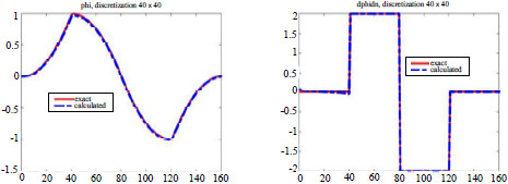
Figure 6.7. Example of numerical solution by Green’s function (example 6.5). For a color version of this figure, see www.iste.co.uk/souzadecursi/variational.zip