
Chapter 3. Getting started with graphs
- Creating and saving graphs
- Customizing symbols, lines, colors, and axes
- Annotating with text and titles
- Controlling a graph’s dimensions
- Combining multiple graphs into one
On many occasions, I’ve presented clients with carefully crafted statistical results in the form of numbers and text, only to have their eyes glaze over while the chirping of crickets permeated the room. Yet those same clients had enthusiastic “Ah-ha!” moments when I presented the same information to them in the form of graphs. Many times I was able to see patterns in data or detect anomalies in data values by looking at graphs—patterns or anomalies that I completely missed when conducting more formal statistical analyses.
Human beings are remarkably adept at discerning relationships from visual representations. A well-crafted graph can help you make meaningful comparisons among thousands of pieces of information, extracting patterns not easily found through other methods. This is one reason why advances in the field of statistical graphics have had such a major impact on data analysis. Data analysts need to look at their data, and this is one area where R shines.
In this chapter, we’ll review general methods for working with graphs. We’ll start with how to create and save graphs. Then we’ll look at how to modify the features that are found in any graph. These features include graph titles, axes, labels, colors, lines, symbols, and text annotations. Our focus will be on generic techniques that apply across graphs. (In later chapters, we’ll focus on specific types of graphs.) Finally, we’ll investigate ways to combine multiple graphs into one overall graph.
3.1. Working with graphs
R is an amazing platform for building graphs. I’m using the term “building” intentionally. In a typical interactive session, you build a graph one statement at a time, adding features, until you have what you want.
Consider the following five lines:
attach(mtcars)
plot(wt, mpg)
abline(lm(mpg~wt))
title("Regression of MPG on Weight")
detach(mtcars)
The first statement attaches the data frame mtcars. The second statement opens a graphics window and generates a scatter plot between automobile weight on the horizontal axis and miles per gallon on the vertical axis. The third statement adds a line of best fit. The fourth statement adds a title. The final statement detaches the data frame. In R, graphs are typically created in this interactive fashion (see figure 3.1).
Figure 3.1. Creating a graph

You can save your graphs via code or through GUI menus. To save a graph via code, sandwich the statements that produce the graph between a statement that sets a destination and a statement that closes that destination. For example, the following will save the graph as a PDF document named mygraph.pdf in the current working directory:
pdf("mygraph.pdf")
 attach(mtcars)
 plot(wt, mpg)
 abline(lm(mpg~wt))
 title("Regression of MPG on Weight")
 detach(mtcars)
dev.off()
In addition to pdf(), you can use the functions win.metafile(), png(), jpeg(), bmp(), tiff(), xfig(), and postscript() to save graphs in other formats. (Note: The Windows metafile format is only available on Windows platforms.) See chapter 1, section 1.3.4 for more details on sending graphic output to files.
Saving graphs via the GUI will be platform specific. On a Windows platform, select File > Save As from the graphics window, and choose the format and location desired in the resulting dialog. On a Mac, choose File > Save As from the menu bar when the Quartz graphics window is highlighted. The only output format provided is PDF. On a Unix platform, the graphs must be saved via code. In appendix A, we’ll consider alternative GUIs for each platform that will give you more options.
Creating a new graph by issuing a high-level plotting command such as plot(), hist() (for histograms), or boxplot() will typically overwrite a previous graph. How can you create more than one graph and still have access to each? There are several methods.
First, you can open a new graph window before creating a new graph:
dev.new()
 statements to create graph 1
dev.new()
 statements to create a graph 2
etc.
Each new graph will appear in the most recently opened window.
Second, you can access multiple graphs via the GUI. On a Mac platform, you can step through the graphs at any time using Back and Forward on the Quartz menu. On a Windows platform, you must use a two-step process. After opening the first graph window, choose History > Recording. Then use the Previous and Next menu items to step through the graphs that are created.
Third and finally, you can use the functions dev.new(), dev.next(), dev.prev(), dev.set(), and dev.off() to have multiple graph windows open at one time and choose which output are sent to which windows. This approach works on any platform. See help(dev.cur) for details on this approach.
R will create attractive graphs with a minimum of input on our part. But you can also use graphical parameters to specify fonts, colors, line styles, axes, reference lines, and annotations. This flexibility allows for a wide degree of customization.
In this chapter, we’ll start with a simple graph and explore the ways you can modify and enhance it to meet your needs. Then we’ll look at more complex examples that illustrate additional customization methods. The focus will be on techniques that you can apply to a wide range of the graphs that you’ll create in R. The methods discussed here will work on all the graphs described in this book, with the exception of those created with the lattice package in chapter 16. (The lattice package has its own methods for customizing a graph’s appearance.) In other chapters, we’ll explore each specific type of graph and discuss where and when they’re most useful.
3.2. A simple example
Let’s start with the simple fictitious dataset given in table 3.1. It describes patient response to two drugs at five dosage levels.
Table 3.1. Patient response to two drugs at five dosage levels
|
Dosage |
Response to Drug A |
Response to Drug B |
|---|---|---|
| 20 | 16 | 15 |
| 30 | 20 | 18 |
| 40 | 27 | 25 |
| 45 | 40 | 31 |
| 60 | 60 | 40 |
You can input this data using this code:
dose  <- c(20, 30, 40, 45, 60)
drugA <- c(16, 20, 27, 40, 60)
drugB <- c(15, 18, 25, 31, 40)
A simple line graph relating dose to response for drug A can be created using
plot(dose, drugA, type="b")
plot() is a generic function that plots objects in R (its output will vary according to the type of object being plotted). In this case, plot(x, y, type="b") places x on the horizontal axis and y on the vertical axis, plots the (x, y) data points, and connects them with line segments. The option type="b" indicates that both points and lines should be plotted. Use help(plot) to view other options. The graph is displayed in figure 3.2.
Figure 3.2. Line plot of dose vs. response for drug A
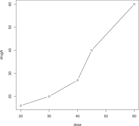
Line plots are covered in detail in chapter 11. Now let’s modify the appearance of this graph.
3.3. Graphical parameters
You can customize many features of a graph (fonts, colors, axes, titles) through options called graphical parameters.
One way is to specify these options through the par() function. Values set in this manner will be in effect for the rest of the session or until they’re changed. The format is par(optionname=value, optionname=value, ...). Specifying par() without parameters produces a list of the current graphical settings. Adding the no.readonly=TRUE option produces a list of current graphical settings that can be modified.
Continuing our example, let’s say that you’d like to use a solid triangle rather than an open circle as your plotting symbol, and connect points using a dashed line rather than a solid line. You can do so with the following code:
opar <- par(no.readonly=TRUE)
par(lty=2, pch=17)
plot(dose, drugA, type="b")
par(opar)
The resulting graph is shown in figure 3.3.
Figure 3.3. Line plot of dose vs. response for drug A with modified line type and symbol

The first statement makes a copy of the current settings. The second statement changes the default line type to dashed (lty=2) and the default symbol for plotting points to a solid triangle (pch=17). You then generate the plot and restore the original settings. Line types and symbols are covered in section 3.3.1.
You can have as many par() functions as desired, so par(lty=2, pch=17) could also have been written as
par(lty=2)
par(pch=17)
A second way to specify graphical parameters is by providing the optionname=value pairs directly to a high-level plotting function. In this case, the options are only in effect for that specific graph. You could’ve generated the same graph with the code
plot(dose, drugA, type="b", lty=2, pch=17)
Not all high-level plotting functions allow you to specify all possible graphical parameters. See the help for a specific plotting function (such as ?plot, ?hist, or ?boxplot) to determine which graphical parameters can be set in this way. The remainder of section 3.3 describes many of the important graphical parameters that you can set.
3.3.1. Symbols and lines
As you’ve seen, you can use graphical parameters to specify the plotting symbols and lines used in your graphs. The relevant parameters are shown in table 3.2.
Table 3.2. Parameters for specifying symbols and lines
|
Parameter |
Description |
|---|---|
| pch | Specifies the symbol to use when plotting points (see figure 3.4). |
| cex | Specifies the symbol size. cex is a number indicating the amount by which plotting symbols should be scaled relative to the default. 1=default, 1.5 is 50% larger, 0.5 is 50% smaller, and so forth. |
| lty | Specifies the line type (see figure 3.5). |
| lwd | Specifies the line width. lwd is expressed relative to the default (default=1). For example, lwd=2 generates a line twice as wide as the default. |
The pch= option specifies the symbols to use when plotting points. Possible values are shown in figure 3.4.
Figure 3.4. Plotting symbols specified with the pch parameter

For symbols 21 through 25 you can also specify the border (col=) and fill (bg=) colors.
Use lty= to specify the type of line desired. The option values are shown in figure 3.5.
Figure 3.5. Line types specified with the lty parameter

Taking these options together, the code
plot(dose, drugA, type="b", lty=3, lwd=3, pch=15, cex=2)
would produce a plot with a dotted line that was three times wider than the default width, connecting points displayed as filled squares that are twice as large as the default symbol size. The results are displayed in figure 3.6.
Figure 3.6. Line plot of dose vs. response for drug A with modified line type, line width, symbol, and symbol width

Next, let’s look at specifying colors.
3.3.2. Colors
There are several color-related parameters in R. Table 3.3 shows some of the common ones.
Table 3.3. Parameters for specifying color
|
Parameter |
Description |
|---|---|
| col | Default plotting color. Some functions (such as lines and pie) accept a vector of values that are recycled. For example, if col=c("red", "blue") and three lines are plotted, the first line will be red, the second blue, and the third red. |
| col.axis | Color for axis text. |
| col.lab | Color for axis labels. |
| col.main | Color for titles. |
| col.sub | Color for subtitles. |
| fg | The plot’s foreground color. |
| bg | The plot’s background color. |
You can specify colors in R by index, name, hexadecimal, RGB, or HSV. For example, col=1, col="white", col="#FFFFFF", col=rgb(1,1,1), and col=hsv(0,0,1) are equivalent ways of specifying the color white. The function rgb() creates colors based on red-green-blue values, whereas hsv() creates colors based on hue-saturation values. See the help feature on these functions for more details.
The function colors() returns all available color names. Earl F. Glynn has created an excellent online chart of R colors, available at http://research.stowers-institute.org/efg/R/Color/Chart. R also has a number of functions that can be used to create vectors of contiguous colors. These include rainbow(), heat.colors(), terrain.colors(), topo.colors(), and cm.colors(). For example, rainbow(10) produces 10 contiguous “rainbow” colors. Gray levels are generated with the gray() function. In this case, you specify gray levels as a vector of numbers between 0 and 1. gray(0:10/10) would produce 10 gray levels. Try the code
n <- 10
mycolors <- rainbow(n)
pie(rep(1, n), labels=mycolors, col=mycolors)
mygrays <- gray(0:n/n)
pie(rep(1, n), labels=mygrays, col=mygrays)
to see how this works. You’ll see examples that use color parameters throughout this chapter.
3.3.3. Text characteristics
Graphic parameters are also used to specify text size, font, and style. Parameters controlling text size are explained in table 3.4. Font family and style can be controlled with font options (see table 3.5).
Table 3.4. Parameters specifying text size
|
Parameter |
Description |
|---|---|
| cex | Number indicating the amount by which plotted text should be scaled relative to the default. 1=default, 1.5 is 50% larger, 0.5 is 50% smaller, etc. |
| cex.axis | Magnification of axis text relative to cex. |
| cex.lab | Magnification of axis labels relative to cex. |
| cex.main | Magnification of titles relative to cex. |
| cex.sub | Magnification of subtitles relative to cex. |
Table 3.5. Parameters specifying font family, size, and style
|
Parameter |
Description |
|---|---|
| font | Integer specifying font to use for plotted text.. 1=plain, 2=bold, 3=italic, 4=bold italic, 5=symbol (in Adobe symbol encoding). |
| font.axis | Font for axis text. |
| font.lab | Font for axis labels. |
| font.main | Font for titles. |
| font.sub | Font for subtitles. |
| ps | Font point size (roughly 1/72 inch). The text size = ps*cex. |
| family | Font family for drawing text. Standard values are serif, sans, and mono. |
For example, all graphs created after the statement
par(font.lab=3, cex.lab=1.5, font.main=4, cex.main=2)
will have italic axis labels that are 1.5 times the default text size, and bold italic titles that are twice the default text size.
Whereas font size and style are easily set, font family is a bit more complicated. This is because the mapping of serif, sans, and mono are device dependent. For example, on Windows platforms, mono is mapped to TT Courier New, serif is mapped to TT Times New Roman, and sans is mapped to TT Arial (TT stands for True Type). If you’re satisfied with this mapping, you can use parameters like family="serif" to get the results you want. If not, you need to create a new mapping. On Windows, you can create this mapping via the windowsFont() function. For example, after issuing the statement
windowsFonts(
  A=windowsFont("Arial Black"),
  B=windowsFont("Bookman Old Style"),
  C=windowsFont("Comic Sans MS")
)
you can use A, B, and C as family values. In this case, par(family="A") will specify an Arial Black font. (Listing 3.2 in section 3.4.2 provides an example of modifying text parameters.) Note that the windowsFont() function only works for Windows. On a Mac, use quartzFonts() instead.
If graphs will be output in PDF or PostScript format, changing the font family is relatively straightforward. For PDFs, use names(pdfFonts()) to find out which fonts are available on your system and pdf(file="myplot.pdf", family=" fontname") to generate the plots. For graphs that are output in PostScript format, use names(postscriptFonts()) and postscript(file="myplot.ps", family=" fontname"). See the online help for more information.
3.3.4. Graph and margin dimensions
Finally, you can control the plot dimensions and margin sizes using the parameters listed in table 3.6.
Table 3.6. Parameters for graph and margin dimensions
|
Parameter |
Description |
|---|---|
| pin | Plot dimensions (width, height) in inches. |
| mai | Numerical vector indicating margin size where c(bottom, left, top, right) is expressed in inches. |
| mar | Numerical vector indicating margin size where c(bottom, left, top, right) is expressed in lines. The default is c(5, 4, 4, 2) + 0.1. |
par(pin=c(4,3), mai=c(1,.5, 1, .2))
produces graphs that are 4 inches wide by 3 inches tall, with a 1-inch margin on the bottom and top, a 0.5-inch margin on the left, and a 0.2-inch margin on the right. For a complete tutorial on margins, see Earl F. Glynn’s comprehensive online tutorial (http://research.stowers-institute.org/efg/R/Graphics/Basics/mar-oma/).
Let’s use the options we’ve covered so far to enhance our simple example. The code in the following listing produces the graphs in figure 3.7.
Figure 3.7. Line plot of dose vs. response for both drug A and drug B

Listing 3.1. Using graphical parameters to control graph appearance
dose  <- c(20, 30, 40, 45, 60)
drugA <- c(16, 20, 27, 40, 60)
drugB <- c(15, 18, 25, 31, 40)
opar <- par(no.readonly=TRUE)
par(pin=c(2, 3))
par(lwd=2, cex=1.5)
par(cex.axis=.75, font.axis=3)
plot(dose, drugA, type="b", pch=19, lty=2, col="red")
plot(dose, drugB, type="b", pch=23, lty=6, col="blue", bg="green")
par(opar)
First you enter your data as vectors, then save the current graphical parameter settings (so that you can restore them later). You modify the default graphical parameters so that graphs will be 2 inches wide by 3 inches tall. Additionally, lines will be twice the default width and symbols will be 1.5 times the default size. Axis text will be set to italic and scaled to 75 percent of the default. The first plot is then created using filled red circles and dashed lines. The second plot is created using filled green filled diamonds and a blue border and blue dashed lines. Finally, you restore the original graphical parameter settings.
Note that parameters set with the par() function apply to both graphs, whereas parameters specified in the plot functions only apply to that specific graph. Looking at figure 3.7 you can see some limitations in your presentation. The graphs lack titles and the vertical axes are not on the same scale, limiting your ability to compare the two drugs directly. The axis labels could also be more informative.
In the next section, we’ll turn to the customization of text annotations (such as titles and labels) and axes. For more information on the graphical parameters that are available, take a look at help(par).
3.4. Adding text, customized axes, and legends
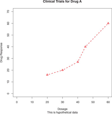
Many high-level plotting functions (for example, plot, hist, boxplot) allow you to include axis and text options, as well as graphical parameters. For example, the following adds a title (main), subtitle (sub), axis labels (xlab, ylab), and axis ranges (xlim, ylim). The results are presented in figure 3.8:
plot(dose, drugA, type="b",
     col="red", lty=2, pch=2, lwd=2,
     main="Clinical Trials for Drug A",
     sub="This is hypothetical data",
     xlab="Dosage", ylab="Drug Response",
     xlim=c(0, 60), ylim=c(0, 70))
Figure 3.8. Line plot of dose versus response for drug A with title, subtitle, and modified axes
Again, not all functions allow you to add these options. See the help for the function of interest to see what options are accepted. For finer control and for modularization, you can use the functions described in the remainder of this section to control titles, axes, legends, and text annotations.
Note
Some high-level plotting functions include default titles and labels. You can remove them by adding ann=FALSE in the plot() statement or in a separate par() statement.
3.4.1. Titles
Use the title() function to add title and axis labels to a plot. The format is
title(main="main title", sub="sub-title",
      xlab="x-axis label", ylab="y-axis label")
Graphical parameters (such as text size, font, rotation, and color) can also be specified in the title() function. For example, the following produces a red title and a blue subtitle, and creates green x and y labels that are 25 percent smaller than the default text size:
title(main="My Title", col.main="red",
      sub="My Sub-title", col.sub="blue",
      xlab="My X label", ylab="My Y label",
      col.lab="green", cex.lab=0.75)
3.4.2. Axes
Rather than using R’s default axes, you can create custom axes with the axis() function. The format is
axis(side, at=, labels=, pos=, lty=, col=, las=, tck=, ...)
where each parameter is described in table 3.7.
Table 3.7. Axis options
|
Option |
Description |
|---|---|
| side | An integer indicating the side of the graph to draw the axis (1=bottom, 2=left, 3=top, 4=right). |
| at | A numeric vector indicating where tick marks should be drawn. |
| labels | A character vector of labels to be placed at the tick marks (if NULL, the at values will be used). |
| pos | The coordinate at which the axis line is to be drawn (that is, the value on the other axis where it crosses). |
| lty | Line type. |
| col | The line and tick mark color. |
| las | Labels are parallel (=0) or perpendicular (=2) to the axis. |
| tck | Length of tick mark as a fraction of the plotting region (a negative number is outside the graph, a positive number is inside, 0 suppresses ticks, 1 creates gridlines); the default is –0.01. |
| (...) | Other graphical parameters. |
When creating a custom axis, you should suppress the axis automatically generated by the high-level plotting function. The option axes=FALSE suppresses all axes (including all axis frame lines, unless you add the option frame.plot=TRUE). The options xaxt="n" and yaxt="n" suppress the x- and y-axis, respectively (leaving the frame lines, without ticks). The following listing is a somewhat silly and overblown example that demonstrates each of the features we’ve discussed so far. The resulting graph is presented in figure 3.9.
Figure 3.9. A demonstration of axis options

Listing 3.2. An example of custom axes

At this point, we’ve covered everything in listing 3.2 except for the line() and the mtext() statements. A plot() statement starts a new graph. By using the line() statement instead, you can add new graph elements to an existing graph. You’ll use it again when you plot the response of drug A and drug B on the same graph in section 3.4.4. The mtext() function is used to add text to the margins of the plot. The mtext() function is covered in section 3.4.5, and the line() function is covered more fully in chapter 11.
Minor Tick Marks
Notice that each of the graphs you’ve created so far have major tick marks but not minor tick marks. To create minor tick marks, you’ll need the minor.tick() function in the Hmisc package. If you don’t already have Hmisc installed, be sure to install it first (see chapter 1, section 1.4.2). You can add minor tick marks with the code
library(Hmisc)
minor.tick(nx=n, ny=n, tick.ratio=n)
where nx and ny specify the number of intervals in which to divide the area between major tick marks on the x-axis and y-axis, respectively. tick.ratio is the size of the minor tick mark relative to the major tick mark. The current length of the major tick mark can be retrieved using par("tck"). For example, the following statement will add one tick mark between each major tick mark on the x-axis and two tick marks between each major tick mark on the y-axis:
minor.tick(nx=2, ny=3, tick.ratio=0.5)
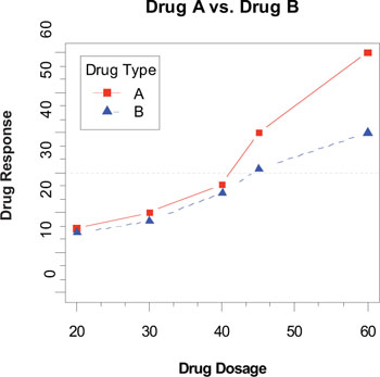
The length of the tick marks will be 50 percent as long as the major tick marks. An example of minor tick marks is given in the next section (listing 3.3 and figure 3.10).
Figure 3.10. An annotated comparison of Drug A and Drug B
3.4.3. Reference lines
The abline() function is used to add reference lines to our graph. The format is
abline(h=yvalues, v=xvalues)
Other graphical parameters (such as line type, color, and width) can also be specified in the abline() function. For example:
abline(h=c(1,5,7))
adds solid horizontal lines at y = 1, 5, and 7, whereas the code
abline(v=seq(1, 10, 2), lty=2, col="blue")
adds dashed blue vertical lines at x = 1, 3, 5, 7, and 9. Listing 3.3 creates a reference line for our drug example at y = 30. The resulting graph is displayed in figure 3.10.
3.4.4. Legend
When more than one set of data or group is incorporated into a graph, a legend can help you to identify what’s being represented by each bar, pie slice, or line. A legend can be added (not surprisingly) with the legend() function. The format is
legend(location, title, legend, ...)
The common options are described in table 3.8.
Table 3.8. Legend options
Other common legend options include bty for box type, bg for background color, cex for size, and text.col for text color. Specifying horiz=TRUE sets the legend horizontally rather than vertically. For more on legends, see help(legend). The examples in the help file are particularly informative.
Let’s take a look at an example using our drug data (listing 3.3). Again, you’ll use a number of the features that we’ve covered up to this point. The resulting graph is presented in figure 3.10.
Listing 3.3. Comparing Drug A and Drug B response by dose

Almost all aspects of the graph in figure 3.10 can be modified using the options discussed in this chapter. Additionally, there are many ways to specify the options desired. The final annotation to consider is the addition of text to the plot itself. This topic is covered in the next section.
3.4.5. Text annotations
Text can be added to graphs using the text() and mtext() functions. text() places text within the graph whereas mtext() places text in one of the four margins. The formats are
text(location, "text to place", pos, ...)
mtext("text to place", side, line=n, ...)
and the common options are described in table 3.9.
Table 3.9. Options for the text() and mtext() functions
|
Option |
Description |
|---|---|
| location | Location can be an x,y coordinate. Alternatively, the text can be placed interactively via mouse by specifying location as locator(1). |
| pos | Position relative to location. 1 = below, 2 = left, 3 = above, 4 = right. If you specify pos, you can specify offset= in percent of character width. |
| side | Which margin to place text in, where 1 = bottom, 2 = left, 3 = top, 4 = right. You can specify line= to indicate the line in the margin starting with 0 (closest to the plot area) and moving out. You can also specify adj=0 for left/bottom alignment or adj=1 for top/right alignment. |
Other common options are cex, col, and font (for size, color, and font style, respectively).
The text() function is typically used for labeling points as well as for adding other text annotations. Specify location as a set of x, y coordinates and specify the text to place as a vector of labels. The x, y, and label vectors should all be the same length. An example is given next and the resulting graph is shown in figure 3.11.
attach(mtcars)
plot(wt, mpg,
     main="Mileage vs. Car Weight",
     xlab="Weight", ylab="Mileage",
     pch=18, col="blue")
text(wt, mpg,
     row.names(mtcars),
     cex=0.6, pos=4, col="red")
detach(mtcars)
Figure 3.11. Example of a scatter plot (car weight vs. mileage) with labeled points (car make)

Here we’ve plotted car mileage versus car weight for the 32 automobile makes provided in the mtcars data frame. The text() function is used to add the car makes to the right of each data point. The point labels are shrunk by 40 percent and presented in red.
As a second example, the following code can be used to display font families:
opar <- par(no.readonly=TRUE)
par(cex=1.5)
plot(1:7,1:7,type="n")
text(3,3,"Example of default text")
text(4,4,family="mono","Example of mono-spaced text")
text(5,5,family="serif","Example of serif text")
par(opar)
The results, produced on a Windows platform, are shown in figure 3.12. Here the par() function was used to increase the font size to produce a better display.
Figure 3.12. Examples of font families on a Windows platform

The resulting plot will differ from platform to platform, because plain, mono, and serif text are mapped to different font families on different systems. What does it look like on yours?
Math Annotations
Finally, you can add mathematical symbols and formulas to a graph using TEX-like rules. See help(plotmath) for details and examples. You can also try demo(plotmath) to see this in action. A portion of the results is presented in figure 3.13. The plotmath() function can be used to add mathematical symbols to titles, axis labels, or text annotation in the body or margins of the graph.
Figure 3.13. Partial results from demo(plotmath)

You can often gain greater insight into your data by comparing several graphs at one time. So, we’ll end this chapter by looking at ways to combine more than one graph into a single image.
3.5. Combining graphs
R makes it easy to combine several graphs into one overall graph, using either the par() or layout() function. At this point, don’t worry about the specific types of graphs being combined; our focus here is on the general methods used to combine them. The creation and interpretation of each graph type is covered in later chapters.
With the par() function, you can include the graphical parameter mfrow=c(nrows, ncols) to create a matrix of nrows × ncols plots that are filled in by row. Alternatively, you can use mfcol=c(nrows, ncols) to fill the matrix by columns.
For example, the following code creates four plots and arranges them into two rows and two columns:
attach(mtcars)
opar <- par(no.readonly=TRUE)
par(mfrow=c(2,2))
plot(wt,mpg, main="Scatterplot of wt vs. mpg")
plot(wt,disp, main="Scatterplot of wt vs disp")
hist(wt, main="Histogram of wt")
boxplot(wt, main="Boxplot of wt")
par(opar)
detach(mtcars)
The results are presented in figure 3.14.
Figure 3.14. Graph combining four figures through par(mfrow=c(2,2))

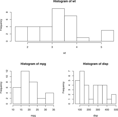
As a second example, let’s arrange 3 plots in 3 rows and 1 column. Here’s the code:
attach(mtcars)
opar <- par(no.readonly=TRUE)
par(mfrow=c(3,1))
hist(wt)
hist(mpg)
hist(disp)
par(opar)
detach(mtcars)
The graph is displayed in figure 3.15. Note that the high-level function hist() includes a default title (use main="" to suppress it, or ann=FALSE to suppress all titles and labels).
Figure 3.15. Graph combining with three figures through par(mfrow=c(3,1))

The layout() function has the form layout(mat) where mat is a matrix object specifying the location of the multiple plots to combine. In the following code, one figure is placed in row 1 and two figures are placed in row 2:
attach(mtcars)
layout(matrix(c(1,1,2,3), 2, 2, byrow = TRUE))
hist(wt)
hist(mpg)
hist(disp)
detach(mtcars)
The resulting graph is presented in figure 3.16.
Figure 3.16. Graph combining three figures using the layout() function with default widths
Optionally, you can include widths= and heights= options in the layout() function to control the size of each figure more precisely. These options have the form
widths = a vector of values for the widths of columns
heights = a vector of values for the heights of rows
Relative widths are specified with numeric values. Absolute widths (in centimeters) are specified with the lcm() function.
In the following code, one figure is again placed in row 1 and two figures are placed in row 2. But the figure in row 1 is one-third the height of the figures in row 2. Additionally, the figure in the bottom-right cell is one-fourth the width of the figure in the bottom-left cell:
attach(mtcars)
layout(matrix(c(1, 1, 2, 3), 2, 2, byrow = TRUE),
       widths=c(3, 1), heights=c(1, 2))
hist(wt)
hist(mpg)
hist(disp)
detach(mtcars)
The graph is presented in figure 3.17.
Figure 3.17. Graph combining three figures using the layout() function with specified widths

As you can see, the layout() function gives you easy control over both the number and placement of graphs in a final image and the relative sizes of these graphs. See help(layout) for more details.
3.5.1. Creating a figure arrangement with fine control
There are times when you want to arrange or superimpose several figures to create a single meaningful plot. Doing so requires fine control over the placement of the figures. You can accomplish this with the fig= graphical parameter. In the following listing, two box plots are added to a scatter plot to create a single enhanced graph. The resulting graph is shown in figure 3.18.
Figure 3.18. A scatter plot with two box plots added to the margins

Listing 3.4. Fine placement of figures in a graph

To understand how this graph was created, think of the full graph area as going from (0,0) in the lower-left corner to (1,1) in the upper-right corner. Figure 3.19 will help you visualize this. The format of the fig= parameter is a numerical vector of the form c(x1, x2, y1, y2).
Figure 3.19. Specifying locations using the fig= graphical parameter
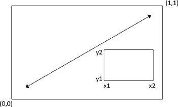
The first fig= sets up the scatter plot going from 0 to 0.8 on the x-axis and 0 to 0.8 on the y-axis. The top box plot goes from 0 to 0.8 on the x-axis and 0.55 to 1 on the y-axis. The right-hand box plot goes from 0.65 to 1 on the x-axis and 0 to 0.8 on the y-axis. fig= starts a new plot, so when adding a figure to an existing graph, include the new=TRUE option.
I chose 0.55 rather than 0.8 so that the top figure would be pulled closer to the scatter plot. Similarly, I chose 0.65 to pull the right-hand box plot closer to the scatter plot. You have to experiment to get the placement right.
Note
The amount of space needed for individual subplots can be device dependent. If you get “Error in plot.new(): figure margins too large,” try varying the area given for each portion of the overall graph.
You can use fig= graphical parameter to combine several plots into any arrangement within a single graph. With a little practice, this approach gives you a great deal of flexibility when creating complex visual presentations.
3.6. Summary
In this chapter, we reviewed methods for creating graphs and saving them in a variety of formats. The majority of the chapter was concerned with modifying the default graphs produced by R, in order to arrive at more useful or attractive plots. You learned how to modify a graph’s axes, fonts, symbols, lines, and colors, as well as how to add titles, subtitles, labels, plotted text, legends, and reference lines. You saw how to specify the size of the graph and margins, and how to combine multiple graphs into a single useful image.
Our focus in this chapter was on general techniques that you can apply to all graphs (with the exception of lattice graphs in chapter 16). Later chapters look at specific types of graphs. For example, chapter 7 covers methods for graphing a single variable. Graphing relationships between variables will be described in chapter 11. In chapter 16, we discuss advanced graphic methods, including lattice graphs (graphs that display the relationship between variables, for each level of other variables) and interactive graphs. Interactive graphs let you use the mouse to dynamically explore the plotted relationships.
In other chapters, we’ll discuss methods of visualizing data that are particularly useful for the statistical approaches under consideration. Graphs are a central part of modern data analysis, and I’ll endeavor to incorporate them into each of the statistical approaches we discuss.
In the previous chapter we discussed a range of methods for inputting or importing data into R. Unfortunately, in the real world your data is rarely usable in the format in which you first get it. In the next chapter we look at ways to transform and massage our data into a state that’s more useful and conducive to analysis.