Chapter 13. Generalized linear models

 

 

In chapters 8 (regression) and 9 (ANOVA), we explored linear models that can be used to predict a normally distributed response variable from a set of continuous and/or categorical predictor variables. But there are many situations in which it’s unreasonable to assume that the dependent variable is normally distributed (or even continuous). For example:

• The outcome variable may be categorical. Binary variables (for example, yes/ no, passed/failed, lived/died) and polytomous variables (for example, poor/ good/excellent, republican/democrat/independent) are clearly not normally distributed.
• The outcome variable may be a count (for example, number of traffic accidents in a week, number of drinks per day). Such variables take on a limited number of values and are never negative. Additionally, their mean and variance are often related (which isn’t true for normally distributed variables).

Generalized linear models extend the linear model framework to include dependent variables that are decidedly non-normal.

In this chapter, we’ll start with a brief overview of generalized linear models and the glm() function used to estimate them. Then we’ll focus on two popular models within this framework: logistic regression (where the dependent variable is categorical) and Poisson regression (where the dependent variable is a count variable).

To motivate the discussion, we’ll apply generalized linear models to two research questions that aren’t easily addressed with standard linear models:

• What personal, demographic, and relationship variables predict marital infidelity? In this case, the outcome variable is binary (affair/no affair).
• What impact does a drug treatment for seizures have on the number of seizures experienced over an eight-week period? In this case, the outcome variable is a count (number of seizures).

We’ll apply logistic regression to address the first question and Poisson regression to address the second. Along the way, we’ll consider extensions of each technique.

13.1. Generalized linear models and the glm() function

A wide range of popular data analytic methods are subsumed within the framework of the generalized linear model. In this section we’ll briefly explore some of the theory behind this approach. You can safely skip over this section if you like and come back to it later.

Let’s say that you want to model the relationship between a response variable Y and a set of p predictor variables X₁ ... X_p. In the standard linear model, you assume that Y is normally distributed and that the form of the relationship is

This equation states that the conditional mean of the response variable is a linear combination of the predictor variables. The β_j are the parameters specifying the expected change in Y for a unit change in X_j and β₀ is the expected value of Y when all the predictor variables are 0. You’re saying that you can predict the mean of the Y distribution for observations with a given set of X values by applying the proper weights to the X variables and adding them up.

Note that you’ve made no distributional assumptions about the predictor variables, X_j.. Unlike Y, there’s no requirement that they be normally distributed. In fact, they’re often categorical (for example, ANOVA designs). Additionally, nonlinear functions of the predictors are allowed. You often include such predictors as X² or X₁ × X₂. What is important is that the equation is linear in the parameters (β₀, β₁,... β_p).

In generalized linear models, you fit models of the form

where g(µ_Y) is a function of the conditional mean (called the link function). Additionally, you relax the assumption that Y is normally distributed. Instead, you assume that Y follows a distribution that’s a member of the exponential family. You specify the link function and the probability distribution, and the parameters are derived through an iterative maximum likelihood estimation procedure.

13.1.1. The glm() function

Generalized linear models are typically fit in R through the glm() function (although other specialized functions are available). The form of the function is similar to lm() but includes additional parameters. The basic format of the function is

glm(formula, family= family (link= function), data=)

where the probability distribution (family) and corresponding default link function (function) are given in table 13.1.

Table 13.1. glm() parameters

Family	Default link function
binomial	(link = "logit")
gaussian	(link = "identity")
gamma	(link = "inverse")
inverse.gaussian	(link = "1/mu^2")
poisson	(link = "log")
quasi	(link = "identity", variance = "constant")
quasibinomial	(link = "logit")
quasipoisson	(link = "log")

The glm() function allows you to fit a number of popular models, including logistic regression, Poisson regression, and survival analysis (not considered here). You can demonstrate this for the first two models as follows. Assume that you have a single response variable (Y), three predictor variables (X1, X2, X3), and a data frame (my-data) containing the data.

Logistic regression is applied to situations in which the response variable is dichotomous (0,1). The model assumes that Y follows a binomial distribution, and that you can fit a linear model of the form

where π = μ_Y, is the conditional mean of Y (that is, the probability that Y = 1 given a set of X values), (π/1 - π) is the odds that Y = 1, and log(π/1 - π) is the log odds, or logit. In this case, log(π/1 - π) is the link function, the probability distribution is binomial, and the logistic regression model can be fit using

glm(Y~X1+X2+X3, family=binomial(link="logit"), data=mydata)

Logistic regression is described more fully in section 13.2.

Poisson regression is applied to situations in which the response variable is the number of events to occur in a given period of time. The Poisson regression model assumes that Y follows a Poisson distribution, and that you can fit a linear model of the form

where λ is the mean (and variance) of Y. In this case, the link function is log(λ), the probability distribution is Poisson, and the Poisson regression model can be fit using

glm(Y~X1+X2+X3, family=poisson(link="log"), data=mydata)

Poisson regression is described in section 13.3.

It is worth noting that the standard linear model is also a special case of the generalized linear model. If you let the link function g(m_Y) = m_Y or the identity function and specify that the probability distribution is normal (Gaussian), then

glm(Y~X1+X2+X3, family=gaussian(link="identity"), data=mydata)

would produce the same results as

lm(Y~X1+X2+X3, data=mydata)

To summarize, generalized linear models extend the standard linear model by fitting a function of the conditional mean response (rather than the conditional mean response), and assuming that the response variable follows a member of the exponential family of distributions (rather than being limited to the normal distribution). The parameter estimates are derived via maximum likelihood rather than least squares.

13.1.2. Supporting functions

Many of the functions that you used in conjunction with lm() when analyzing standard linear models have corresponding versions for glm(). Some commonly used functions are given in table 13.2.

Table 13.2. Functions that support glm()

Function	Description
summary()	Displays detailed results for the fitted model
coefficients(), coef()	Lists the model parameters (intercept and slopes) for the fitted model
confint()	Provides confidence intervals for the model parameters (95 percent by default)
residuals()	Lists the residual values for a fitted model
anova()	Generates an ANOVA table comparing two fitted models
plot()	Generates diagnostic plots for evaluating the fit of a model
predict()	Uses a fitted model to predict response values for a new dataset

We’ll explore examples of these functions in later sections. In the next section, we’ll briefly consider the assessment of model adequacy.

13.1.3. Model fit and regression diagnostics

The assessment of model adequacy is as important for generalized linear models as it is for standard (OLS) linear models. Unfortunately, there’s less agreement in the statistical community regarding appropriate assessment procedures. In general, you can use the techniques described in chapter 8, with the following caveats.

When assessing model adequacy, you’ll typically want to plot predicted values expressed in the metric of the original response variable against residuals of the deviance type. For example, a common diagnostic plot would be

plot(predict(model, type="response"),
    residuals(model, type= "deviance"))

where model is the object returned by the glm() function.

The hat values, studentized residuals, and Cook’s D statistics that R provides will be approximate values. Additionally, there’s no general consensus on cutoff values for identifying problematic observations. Values have to be judged relative to each other. One approach is to create index plots for each statistic and look for unusually large values. For example, you could use the following code to create three diagnostic plots:

plot(hatvalues(model))
plot(rstudent(model))
plot(cooks.distance(model))

Alternatively, you could use the code

library(car)
influencePlot(model)

to create one omnibus plot. In the latter graph, the horizontal axis is the leverage, the vertical axis is the studentized residual, and the plotted symbol is proportional to the Cook’s distance.

Diagnostic plots tend to be most helpful when the response variable takes on many values. When the response variable can only take on a limited number of values (for example, logistic regression), their utility is decreased.

For more on regression diagnostics for generalized linear models, see Fox (2008) and Faraway (2006). In the remaining portion of this chapter, we’ll consider two of the most popular forms of the generalized linear model in detail: logistic regression and Poisson regression.

13.2. Logistic regression

Logistic regression is useful when predicting a binary outcome from a set of continuous and/or categorical predictor variables. To demonstrate this, we’ll explore the data on infidelity contained in the data frame Affairs, provided with the AER package. Be sure to download and install the package (using install.packages("AER")) before first use.

The infidelity data, known as Fair’s Affairs, is based on a cross-sectional survey conducted by Psychology Today in 1969, and is described in Greene (2003) and Fair (1978). It contains nine variables collected on 601 participants and includes how often the respondent engaged in extramarital sexual intercourse during the past year, as well as their gender, age, years married, whether or not they had children, their religiousness (on a 5-point scale from 1=anti to 5=very), education, occupation (Hollingshead 7-point classification with reverse numbering), and a numeric self-rating of their marriage (from 1=very unhappy to 5=very happy).

Let’s look at some descriptive statistics:

> data(Affairs, package="AER")
> summary(Affairs)
    affairs          gender         age         yearsmarried     children
 Min.   : 0.000   female:315   Min.   :17.50   Min.   : 0.125    no :171
 1st Qu.: 0.000   male  :286   1st Qu.:27.00   1st Qu.: 4.000    yes:430
 Median : 0.000                Median :32.00   Median : 7.000
 Mean   : 1.456                Mean   :32.49   Mean   : 8.178
 3rd Qu.: 0.000                3rd Qu.:37.00   3rd Qu.:15.000
 Max.   :12.000                Max.   :57.00   Max.   :15.000
 religiousness     education       occupation        rating
 Min.   :1.000   Min.   : 9.00   Min.   :1.000   Min.    :1.000
 1st Qu.:2.000   1st Qu.:14.00   1st Qu.:3.000   1st Qu.:3.000
 Median :3.000   Median :16.00   Median :5.000   Median :4.000
 Mean   :3.116   Mean   :16.17   Mean   :4.195   Mean    :3.932
 3rd Qu.:4.000   3rd Qu.:18.00   3rd Qu.:6.000   3rd Qu.:5.000
 Max.   :5.000   Max.   :20.00   Max.   :7.000   Max.    :5.000

> table(Affairs$affairs)
  0   1   2   3   7  12
451  34  17  19  42  38

From these statistics, you can see that that 52 percent of respondents were female, that 72 percent had children, and that the median age for the sample was 32 years. With regard to the response variable, 75 percent of respondents reported not engaging in an infidelity in the past year (451/601). The largest number of encounters reported was 12 (6 percent).

Although the number of indiscretions was recorded, our interest here is in the binary outcome (had an affair/didn’t have an affair). You can transform affairs into a dichotomous factor called ynaffair with the following code.

> Affairs$ynaffair[Affairs$affairs  > 0] <- 1
> Affairs$ynaffair[Affairs$affairs == 0] <- 0
> Affairs$ynaffair <- factor(Affairs$ynaffair,
                             levels=c(0,1),
                             labels=c("No","Yes"))
> table(Affairs$ynaffair)
No Yes
451 150

This dichotomous factor can now be used as the outcome variable in a logistic regression model:

> fit.full <- glm(ynaffair ~ gender + age + yearsmarried + children +
                  religiousness + education + occupation +rating,
                  data=Affairs,family=binomial())
< summary(fit.full)

Call:
glm(formula = ynaffair ~ gender + age + yearsmarried + children +
    religiousness + education + occupation + rating, family = binomial(),
    data = Affairs)

Deviance Residuals:
   Min      1Q  Median      3Q      Max
-1.571  -0.750  -0.569  -0.254    2.519

Coefficients:
              Estimate Std. Error z value Pr(>|z|)
(Intercept)     1.3773     0.8878    1.55  0.12081
gendermale      0.2803     0.2391    1.17  0.24108
age            -0.0443     0.0182   -2.43  0.01530 *
yearsmarried    0.0948     0.0322    2.94  0.00326 **
childrenyes     0.3977     0.2915    1.36  0.17251
religiousness  -0.3247     0.0898   -3.62  0.00030 ***
education       0.0211     0.0505    0.42  0.67685
occupation      0.0309     0.0718    0.43  0.66663
rating         -0.4685     0.0909   -5.15  2.6e-07 ***
---
Signif. codes:  0 '***' 0.001 '**' 0.01 '*' 0.05 '.' 0.1 ' ' 1

(Dispersion parameter for binomial family taken to be 1)

    Null deviance: 675.38  on 600  degrees of freedom
Residual deviance: 609.51  on 592  degrees of freedom
AIC: 627.5

Number of Fisher Scoring iterations: 4

From the p-values for the regression coefficients (last column), you can see that gender, presence of children, education, and occupation may not make a significant contribution to the equation (you can’t reject the hypothesis that the parameters are 0). Let’s fit a second equation without them, and test whether this reduced model fits the data as well:

> fit.reduced <- glm(ynaffair ~ age + yearsmarried + religiousness +
                     rating, data=Affairs, family=binomial())
> summary(fit.reduced)

Call:
glm(formula = ynaffair ~ age + yearsmarried + religiousness + rating,
    family = binomial(), data = Affairs)

Deviance Residuals:
   Min      1Q  Median      3Q      Max
-1.628  -0.755  -0.570  -0.262    2.400

Coefficients:
              Estimate Std. Error z value Pr(>|z|)
(Intercept)     1.9308     0.6103     3.16  0.00156 **
age            -0.0353     0.0174    -2.03  0.04213 *
yearsmarried    0.1006     0.0292     3.44  0.00057 ***
religiousness  -0.3290     0.0895    -3.68  0.00023 ***
rating         -0.4614     0.0888    -5.19  2.1e-07 ***
---
Signif. codes:  0 '***' 0.001 '**' 0.01 '*' 0.05 '.' 0.1 ' ' 1

(Dispersion parameter for binomial family taken to be 1)

    Null deviance: 675.38  on 600  degrees of freedom
Residual deviance: 615.36  on 596  degrees of freedom
AIC: 625.4

Number of Fisher Scoring iterations: 4

Each regression coefficient in the reduced model is statistically significant (p<.05). Because the two models are nested (fit.reduced is a subset of fit.full), you can use the anova() function to compare them. For generalized linear models, you’ll want a chi-square version of this test.

> anova(fit.reduced, fit.full, test="Chisq")
Analysis of Deviance Table

Model 1: ynaffair ~ age + yearsmarried + religiousness + rating
Model 2: ynaffair ~ gender + age + yearsmarried + children +
    religiousness + education + occupation + rating
  Resid. Df Resid. Dev Df Deviance P(>|Chi|)
1       596        615
2       592        610  4     5.85      0.21

The nonsignificant chi-square value (p=0.21) suggests that the reduced model with four predictors fits as well as the full model with nine predictors, reinforcing your belief that gender, children, education, and occupation don’t add significantly to the prediction above and beyond the other variables in the equation. Therefore, you can base your interpretations on the simpler model.

13.2.1. Interpreting the model parameters

Let’s take a look at the regression coefficients:

> coef(fit.reduced)
  (Intercept)           age  yearsmarried religiousness        rating
        1.931        -0.035         0.101        -0.329        -0.461

In a logistic regression, the response being modeled is the log(odds) that Y=1. The regression coefficients give the change in log(odds) in the response for a unit change in the predictor variable, holding all other predictor variables constant.

Because log(odds) are difficult to interpret, you can exponentiate them to put the results on an odds scale:

> exp(coef(fit.reduced))
  (Intercept)           age  yearsmarried religiousness        rating
        6.895         0.965         1.106         0.720         0.630

Now you can see that the odds of an extramarital encounter are increased by a factor of 1.106 for a one-year increase in years married (holding age, religiousness, and marital rating constant). Conversely, the odds of an extramarital affair are multiplied by a factor of 0.965 for every year increase in age. The odds of an extramarital affair increase with years married, and decrease with age, religiousness, and marital rating. Because the predictor variables can’t equal 0, the intercept isn’t meaningful in this case.

If desired, you can use the confint() function to obtain confidence intervals for the coefficients. For example, exp(confint(fit.reduced)) would print 95 percent confidence intervals for each of the coefficients on an odds scale.

Finally, a one-unit change in a predictor variable may not be inherently interesting. For binary logistic regression, the change in the odds of the higher value on the response variable for an n unit change in a predictor variable is exp(β_j)^Λn. If a one-year increase in years married multiplies the odds of an affair by 1.106, a 10-year increase would increase the odds by a factor of 1.106^Λ 10, or 2.7, holding the other predictor variables constant.

13.2.2. Assessing the impact of predictors on the probability of an outcome

For many of us, it’s easier to think in terms of probabilities than odds. You can use the predict() function to observe the impact of varying the levels of a predictor variable on the probability of the outcome. The first step is to create an artificial dataset containing the values of the predictor variables that you’re interested in. Then you can use this artificial dataset with the predict() function to predict the probabilities of the outcome event occurring for these values.

Let’s apply this strategy to assess the impact of marital ratings on the probability of having an extramarital affair. First, create an artificial dataset, where age, years married, and religiousness are set to their means, and marital rating varies from 1 to 5.

> testdata <- data.frame(rating=c(1, 2, 3, 4, 5), age=mean(Affairs$age),
                         yearsmarried=mean(Affairs$yearsmarried),
                         religiousness=mean(Affairs$religiousness))
> testdata
  rating  age yearsmarried religiousness
1      1 32.5         8.18          3.12
2      2 32.5         8.18          3.12
3      3 32.5         8.18          3.12
4      4 32.5         8.18          3.12
5      5 32.5         8.18          3.12

Next, use the test dataset and prediction equation to obtain probabilities:

> testdata$prob <- predict(fit.reduced, newdata=testdata, type="response")
  testdata
  rating  age yearsmarried religiousness  prob
1      1 32.5         8.18          3.12 0.530
2      2 32.5         8.18          3.12 0.416
3      3 32.5         8.18          3.12 0.310
4      4 32.5         8.18          3.12 0.220
5      5 32.5         8.18          3.12 0.151

From these results you see that the probability of an extramarital affair decreases from 0.53 when the marriage is rated 1=very unhappy to 0.15 when the marriage is rated 5=very happy (holding age, years married, and religiousness constant). Now look at the impact of age:

> testdata <- data.frame(rating=mean(Affairs$rating),
                         age=seq(17, 57, 10),
                         yearsmarried=mean(Affairs$yearsmarried),
                         religiousness=mean(Affairs$religiousness))
> testdata
  rating age yearsmarried religiousness
1   3.93  17         8.18          3.12
2   3.93  27         8.18          3.12
3   3.93  37         8.18          3.12
4   3.93  47         8.18          3.12
5   3.93  57         8.18          3.12

> testdata$prob <- predict(fit.reduced, newdata=testdata, type="response")
> testdata
  rating age yearsmarried religiousness     prob
1   3.93  17         8.18          3.12    0.335
2   3.93  27         8.18          3.12    0.262
3   3.93  37         8.18          3.12    0.199
4   3.93  47         8.18          3.12    0.149
5   3.93  57         8.18          3.12    0.109

Here, you see that as age increases from 17 to 57, the probability of an extramarital encounter decreases from 0.34 to 0.11, holding the other variables constant. Using this approach, you can explore the impact of each predictor variable on the outcome.

13.2.3. Overdispersion

The expected variance for data drawn from a binomial distribution is σ² = nπ(l- π), where n is the number of observations and π is the probability of belonging to the Y=1 group. Overdispersion occurs when the observed variance of the response variable is larger than what would be expected from a binomial distribution. Overdispersion can lead to distorted test standard errors and inaccurate tests of significance.

When overdispersion is present, you can still fit a logistic regression using the glm() function, but in this case, you should use the quasibinomial distribution rather than the binomial distribution.

One way to detect overdispersion is to compare the residual deviance with the residual degrees of freedom in your binomial model. If the ratio

is considerably larger than 1, you have evidence of overdispersion. Applying this to the Affairs example, you have

which is close to 1, suggesting no overdispersion.

You can also test for overdispersion. To do this, you fit the model twice, but in the first instance you use family="binomial" and in the second instance you use family="quasibinomial". If the glm() object returned in the first case is called fit and the object returned in the second case is called fit.od, then

pchisq(summary(fit.od)$dispersion * fit$df.residual,
        fit$df.residual, lower = F)

provides the p-value for testing the null hypothesis H₀: Φ = 1 versus the alternative hypothesis H₁: Φ ≠ 1. If p is small (say, less than 0.05), you’d reject the null hypothesis.

Applying this to the Affairs dataset, you have

> fit <- glm(ynaffair ~ age + yearsmarried + religiousness +
             rating, family = binomial(), data = Affairs)
> fit.od <- glm(ynaffair ~ age + yearsmarried + religiousness +
                rating, family = quasibinomial(), data = Affairs)
> pchisq(summary(fit.od)$dispersion * fit$df.residual,
         fit$df.residual, lower = F)

[1] 0.34

The resulting p-value (0.34) is clearly not significant (p>0.05), strengthening our belief that overdispersion isn’t a problem. We’ll return to the issue of overdispersion when we discuss Poisson regression.

13.2.4. Extensions

Several logistic regression extensions and variations are available in R:

• Robust logistic regression—The glmRob() function in the robust package can be used to fit a robust generalized linear model, including robust logistic regression. Robust logistic regression can be helpful when fitting logistic regression models to data containing outliers and influential observations.
• Multinomial logistic regression—If the response variable has more than two unordered categories (for example, married/widowed/divorced), you can fit a polyto-mous logistic regression using the mlogit() function in the mlogit package.
• Ordinal logistic regression—If the response variable is a set of ordered categories (for example, credit risk as poor/good/excellent), you can fit an ordinal logistic regression using the lrm() function in the rms package.

The ability to model a response variable with multiple categories (both ordered and unordered) is an important extension, but it comes at the expense of greater interpretive complexity. Assessing model fit and regression diagnostics in these cases will also be more complex.

In the Affairs example, the number of extramarital contacts was dichotomized into a yes/no response variable because our interest centered on whether respondents had an affair in the past year. If our interest had been centered on magnitude—the number of encounters in the past year—we would have analyzed the count data directly. One popular approach to analyzing count data is Poisson regression, the next topic we’ll address.

13.3. Poisson regression

Poisson regression is useful when you’re predicting an outcome variable representing counts from a set of continuous and/or categorical predictor variables. A comprehensive yet accessible introduction to Poisson regression is provided by Coxe, West, and Aiken (2009).

To illustrate the fitting of a Poisson regression model, along with some issues that can come up in the analysis, we’ll use the Breslow seizure data (Breslow, 1993) provided in the robust package. Specifically, we’ll consider the impact of an antiepileptic drug treatment on the number of seizures occurring over an eight-week period following the initiation of therapy. Be sure to install the robust package before continuing.

Data were collected on the age and number of seizures reported by patients suffering from simple or complex partial seizures during an eight-week period before, and eight-week period after, randomization into a drug or placebo condition. sumY (the number of seizures in the eight-week period post-randomization) is the response variable. Treatment condition (Trt), age in years (Age), and number of seizures reported in the baseline eight-week period (Base) are the predictor variables. The baseline number of seizures and age are included because of their potential effect on the response variable. We are interested in whether or not evidence exists that the drug treatment decreases the number of seizures after accounting for these covariates.

First, let’s look at summary statistics for the dataset:

> data(breslow.dat, package="robust")
> names(breslow.dat)
 [1] "ID"    "Y1"    "Y2"    "Y3"    "Y4"    "Base"  "Age"   "Trt"   "Ysum"
[10] "sumY"  "Age10" "Base4"

> summary(breslow.dat[c(6,7,8,10)])
      Base            Age              Trt          sumY
 Min.   :  6.0   Min.   :18.0   placebo  :28   Min.   :  0.0
 1st Qu.: 12.0   1st Qu.:23.0   progabide:31   1st Qu.: 11.5
 Median : 22.0   Median :28.0                  Median : 16.0
 Mean   : 31.2   Mean   :28.3                  Mean   : 33.1
 3rd Qu.: 41.0   3rd Qu.:32.0                  3rd Qu.: 36.0
 Max.   :151.0   Max.   :42.0                  Max.   :302.0

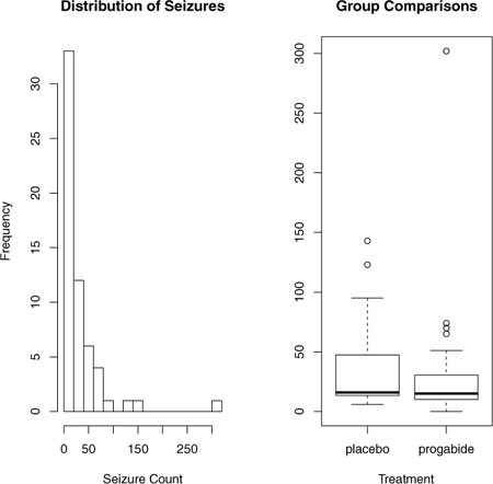
Note that although there are 12 variables in the dataset, we’re limiting our attention to the four described earlier. Both the baseline and post-randomization number of seizures is highly skewed. Let’s look at the response variable in more detail. The following code produces the graphs in figure 13.1.

Figure 13.1. Distribution of post-treatment seizure counts (Source: Breslow seizure data)

opar <- par(no.readonly=TRUE)
par(mfrow=c(1,2))
attach(breslow.dat)
hist(sumY, breaks=20, xlab="Seizure Count",
     main="Distribution of Seizures")
boxplot(sumY ~ Trt, xlab="Treatment", main="Group Comparisons")
par(opar)

You can clearly see the skewed nature of the dependent variable and the possible presence of outliers. At first glance, the number of seizures in the drug condition appears to be smaller and have a smaller variance. (You’d expect a smaller variance to accompany a smaller mean with Poisson distributed data.) Unlike standard OLS regression, this heterogeneity of variance isn’t a problem in Poisson regression.

The next step is to fit the Poisson regression:

> fit <- glm(sumY ~ Base + Age + Trt, data=breslow.dat, family=poisson())
> summary(fit)

Call:
glm(formula = sumY ~ Base + Age + Trt, family = poisson(), data = breslow.
   dat)

Deviance Residuals:
   Min      1Q  Median      3Q      Max
-6.057  -2.043  -0.940    0.793  11.006

Coefficients:
              Estimate Std. Error z value Pr(>|z|)
(Intercept)   1.948826   0.135619    14.37  < 2e-16 ***
Base          0.022652   0.000509    44.48  < 2e-16 ***
Age           0.022740   0.004024     5.65  1.6e-08 ***
Trtprogabide -0.152701   0.047805   -3.19    0.0014 **
---
Signif. codes:  0 '***' 0.001 '**' 0.01 '*' 0.05 '.' 0.1 ' ' 1

(Dispersion parameter for poisson family taken to be 1)

    Null deviance: 2122.73  on 58  degrees of freedom
Residual deviance:  559.44  on 55  degrees of freedom
AIC: 850.7

Number of Fisher Scoring iterations: 5

The output provides the deviances, regression parameters, standard errors, and tests that these parameters are 0. Note that each of the predictor variables is significant at the p<0.05 level.

13.3.1. Interpreting the model parameters

The model coefficients are obtained using the coef() function, or by examining the Coefficients table in the summary() function output:

> coef(fit)
 (Intercept)         Base           Age Trtprogabide
      1.9488       0.0227       0.0227       -0.1527

In a Poisson regression, the dependent variable being modeled is the log of the conditional mean log_e(λ). The regression parameter 0.0227 for Age indicates that a one-year increase in age is associated with a 0.03 increase in the log mean number of seizures, holding baseline seizures and treatment condition constant. The intercept is the log mean number of seizures when each of the predictors equals 0. Because you can’t have a zero age and none of the participants had a zero number of baseline seizures, the intercept isn’t meaningful in this case.

It’s usually much easier to interpret the regression coefficients in the original scale of the dependent variable (number of seizures, rather than log number of seizures). To accomplish this, exponentiate the coefficients:

> exp(coef(fit))
 (Intercept)         Base           Age Trtprogabide
       7.020        1.023        1.023         0.858

Now you see that a one-year increase in age multiplies the expected number of seizures by 1.023, holding the other variables constant. This means that increased age is associated with higher numbers of seizures. More importantly, a one-unit change in Trt (that is, moving from placebo to progabide) multiplies the expected number of seizures by 0.86. You’d expect a 20 percent decrease in the number of seizures for the drug group compared with the placebo group, holding baseline number of seizures and age constant.

It’s important to remember that, like the exponeniated parameters in logistic regression, the exponeniated parameters in the Poisson model have a multiplicative rather than an additive effect on the response variable. Also, as with logistic regression, you must evaluate your model for overdispersion.

13.3.2. Overdispersion

In a Poisson distribution, the variance and mean are equal. Overdispersion occurs in Poisson regression when the observed variance of the response variable is larger than would be predicted by the Poisson distribution. Because overdispersion is often encountered when dealing with count data, and can have a negative impact on the interpretation of the results, we’ll spend some time discussing it.

There are several reasons why overdispersion may occur (Coxe et al., 2009):

• The omission of an important predictor variable can lead to overdispersion.
• Overdispersion can also be caused by a phenomenon known as state dependence. Within observations, each event in a count is assumed to be independent. For the seizure data, this would imply that for any patient, the probability of a seizure is independent of each other seizure. But this assumption is often untenable. For a given individual, the probability of having a first seizure is unlikely to be the same as the probability of having a 40th seizure, given that they’ve already had 39.
• In longitudinal studies, overdispersion can be caused by the clustering inherent in repeated measures data. We won’t discuss longitudinal Poisson models here.

If overdispersion is present and you don’t account for it in your model, you’ll get standard errors and confidence intervals that are too small, and significance tests that are too liberal (that is, you’ll find effects that aren’t really there).

As with logistic regression, overdispersion is suggested if the ratio of the residual deviance to the residual degrees of freedom is much larger than 1. For your seizure data, the ratio is

which is clearly much larger than 1.

The qcc package provides a test for overdispersion in the Poisson case. (Be sure to download and install this package before first use.) You can test for overdispersion in the seizure data using the following code:

> library(qcc)
> qcc.overdispersion.test(breslow.dat$sumY, type="poisson")

Overdispersion test Obs.Var/Theor.Var Statistic p-value
       poisson data              62.9      3646       0

Not surprisingly, the significance test has a p-value less than 0.05, strongly suggesting the presence of overdispersion.

You can still fit a model to your data using the glm() function, by replacing family="poisson" with family="quasipoisson". Doing so is analogous to our approach to logistic regression when overdispersion is present.

> fit.od <- glm(sumY ~ Base + Age + Trt, data=breslow.dat,
                family=quasipoisson())
> summary(fit.od)

Call:
glm(formula = sumY ~ Base + Age + Trt, family = quasipoisson(),
    data = breslow.dat)

Deviance Residuals:
   Min      1Q  Median      3Q      Max
-6.057  -2.043  -0.940    0.793  11.006

Coefficients:
             Estimate Std. Error t value Pr(>|t|)
(Intercept)   1.94883    0.46509    4.19  0.00010 ***
Base          0.02265    0.00175   12.97  < 2e-16 ***
Age           0.02274    0.01380    1.65  0.10509
Trtprogabide -0.15270    0.16394   -0.93  0.35570
---
Signif. codes:  0 '***' 0.001 '**' 0.01 '*' 0.05 '.' 0.1 ' ' 1

(Dispersion parameter for quasipoisson family taken to be 11.8)

    Null deviance: 2122.73  on 58  degrees of freedom
Residual deviance:  559.44  on 55  degrees of freedom
AIC: NA

Number of Fisher Scoring iterations: 5

Notice that the parameter estimates in the quasi-Poisson approach are identical to those produced by the Poisson approach. The standard errors are much larger, though. In this case, the larger standard errors have led to p-values for Trt (and Age) that are greater than 0.05. When you take overdispersion into account, there’s insufficient evidence to declare that the drug regimen reduces seizure counts more than receiving a placebo, after controlling for baseline seizure rate and age.

Please remember that this example is used for demonstration purposes only. The results shouldn’t be taken to imply anything about the efficacy of progabide in the real world. I’m not a doctor—at least not a medical doctor—and I don’t even play one on TV.

We’ll finish this exploration of Poisson regression with a discussion of some important variants and extensions.

13.3.3. Extensions

R provides several useful extensions to the basic Poisson regression model, including models that allow varying time periods, models that correct for too many zeros, and robust models that are useful when data includes outliers and influential observations. I’ll describe each separately.

Poisson Regression with Varying Time Periods

Our discussion of Poisson regression has been limited to response variables that measure a count over a fixed length of time (for example, number of seizures in an eight-week period, number of traffic accidents in the past year, number of pro-social behaviors in a day). The length of time is constant across observations. But you can fit Poisson regression models that allow the time period to vary for each observation. In this case, the outcome variable is a rate.

To analyze rates, you must include a variable (for example, time) that records the length of time over which the count occurs for each observation. You then change your model from

or equivalently to

To fit this new model, you use the offset option in the glm() function. For example, assume that the length of time that patients participated post-randomization in the Breslow study varied from 14 days to 60 days. You could use the rate of seizures as the dependent variable (assuming you had recorded time for each patient in days), and fit the model

fit <- glm(sumY ~ Base + Age + Trt, data=breslow.dat,
           offset= log(time), family=poisson())

where sumY is the number of seizures that occurred post-randomization for a patient during the time the patient was studied. In this case you’re assuming that rate doesn’t vary over time (for example, 2 seizures in 4 days is equivalent to 10 seizures in 20 days).

Zero-Inflated Poisson Regression

There are times when the number of zero counts in a dataset is larger than would be predicted by the Poisson model. This can occur when there’s a subgroup of the population that would never engage in the behavior being counted. For example, in the Affairs dataset described in the section on logistic regression, the original outcome variable (affairs) counted the number of extramarital sexual intercourse experience participants had in the past year. It’s likely that there’s a subgroup of faithful marital partners who would never have an affair, no matter how long the period of time studied. These are called structural zeros (primarily by the swingers in the group).

In such cases, you can analyze the data using an approach called zero-inflated Poisson regression. The approach fits two models simultaneously—one that predicts who would or would not have an affair, and the second that predicts how many affairs a participant would have if you excluded the permanently faithful. Think of this as a model that combines a logistic regression (for predicting structural zeros) and a Poisson regression model (that predicts counts for observations that aren’t structural zeros). Zero-inflated Poisson regression can be fit using the zeroinfl() function in the pscl package.

Robust Poisson Regression

Finally, the glmRob() function in the robust package can be used to fit a robust generalized linear model, including robust Poisson regression. As mentioned previously, this can be helpful in the presence of outliers and influential observations.

 

 

13.4. Summary

In this chapter, we used generalized linear models to expand the range of approaches available for helping you to understand your data. In particular, the framework allows you to analyze response variables that are decidedly non-normal, including categorical outcomes and discrete counts. After briefly describing the general approach, we focused on logistic regression (for analyzing a dichotomous outcome) and Poisson regression (for analyzing outcomes measured as counts or rates).

We also discussed the important topic of overdispersion, including how to detect it and how to adjust for it. Finally, we looked at some of the extensions and variations that are available in R.

Each of the statistical approaches covered so far has dealt with directly observed and recorded variables. In the next chapter, we’ll look at statistical models that deal with latent variables—unobserved, theoretical variables that you believe underlie and account for the behavior of the variables you do observe. In particular, you’ll see how you can use factor analytic methods to detect and test hypotheses about these unobserved variables.