Chapter 8. Regression

 

 

In many ways, regression analysis lives at the heart of statistics. It’s a broad term for a set of methodologies used to predict a response variable (also called a dependent, criterion, or outcome variable) from one or more predictor variables (also called independent or explanatory variables). In general, regression analysis can be used to identify the explanatory variables that are related to a response variable, to describe the form of the relationships involved, and to provide an equation for predicting the response variable from the explanatory variables.

For example, an exercise physiologist might use regression analysis to develop an equation for predicting the expected number of calories a person will burn while exercising on a treadmill. The response variable is the number of calories burned (calculated from the amount of oxygen consumed), and the predictor variables might include duration of exercise (minutes), percentage of time spent at their target heart rate, average speed (mph), age (years), gender, and body mass index (BMI).

From a theoretical point of view, the analysis will help answer such questions as these:

• What’s the relationship between exercise duration and calories burned? Is it linear or curvilinear? For example, does exercise have less impact on the number of calories burned after a certain point?
• How does effort (the percentage of time at the target heart rate, the average walking speed) factor in?
• Are these relationships the same for young and old, male and female, heavy and slim?

From a practical point of view, the analysis will help answer such questions as the following:

• How many calories can a 30-year-old man with a BMI of 28.7 expect to burn if he walks for 45 minutes at an average speed of 4 miles per hour and stays within his target heart rate 80 percent of the time?
• What’s the minimum number of variables you need to collect in order to accurately predict the number of calories a person will burn when walking?
• How accurate will your prediction tend to be?

Because regression analysis plays such a central role in modern statistics, we’ll cover it in some depth in this chapter. First, we’ll look at how to fit and interpret regression models. Next, we’ll review a set of techniques for identifying potential problems with these models and how to deal with them. Third, we’ll explore the issue of variable selection. Of all the potential predictor variables available, how do you decide which ones to include in your final model? Fourth, we’ll address the question of generalizability. How well will your model work when you apply it in the real world? Finally, we’ll look at the issue of relative importance. Of all the predictors in your model, which one is the most important, the second most important, and the least important?

As you can see, we’re covering a lot of ground. Effective regression analysis is an interactive, holistic process with many steps, and it involves more than a little skill. Rather than break it up into multiple chapters, I’ve opted to present this topic in a single chapter in order to capture this flavor. As a result, this will be the longest and most involved chapter in the book. Stick with it to the end and you’ll have all the tools you need to tackle a wide variety of research questions. Promise!

8.1. The many faces of regression

The term regression can be confusing because there are so many specialized varieties (see table 8.1). In addition, R has powerful and comprehensive features for fitting regression models, and the abundance of options can be confusing as well. For example, in 2005, Vito Ricci created a list of over 205 functions in R that are used to generate regression analyses (http://cran.r-project.org/doc/contrib/Ricci-refcardregression.pdf).

Table 8.1. Varieties of regression analysis

Type of regression	Typical use
Simple linear	Predicting a quantitative response variable from a quantitative explanatory variable
Polynomial	Predicting a quantitative response variable from a quantitative explanatory variable, where the relationship is modeled as an nth order polynomial
Multiple linear	Predicting a quantitative response variable from two or more explanatory variables
Multivariate	Predicting more than one response variable from one or more explanatory variables
Logistic	Predicting a categorical response variable from one or more explanatory variables
Poisson	Predicting a response variable representing counts from one or more explanatory variables
Cox proportional hazards	Predicting time to an event (death, failure, relapse) from one or more explanatory variables
Time-series	Modeling time-series data with correlated errors
Nonlinear	Predicting a quantitative response variable from one or more explanatory variables, where the form of the model is nonlinear
Nonparametric	Predicting a quantitative response variable from one or more explanatory variables, where the form of the model is derived from the data and not specified a priori
Robust	Predicting a quantitative response variable from one or more explanatory variables using an approach that’s resistant to the effect of influential observations

In this chapter, we’ll focus on regression methods that fall under the rubric of ordinary least squares (OLS) regression, including simple linear regression, polynomial regression, and multiple linear regression. OLS regression is the most common variety of statistical analysis today. Other types of regression models (including logistic regression and Poisson regression) will be covered in chapter 13.

8.1.1. Scenarios for using OLS regression

In OLS regression, a quantitative dependent variable is predicted from a weighted sum of predictor variables, where the weights are parameters estimated from the data. Let’s take a look at a concrete example (no pun intended), loosely adapted from Fwa (2006).

An engineer wants to identify the most important factors related to bridge deterioration (such as age, traffic volume, bridge design, construction materials and methods, construction quality, and weather conditions) and determine the mathematical form of these relationships. She collects data on each of these variables from a representative sample of bridges and models the data using OLS regression.

The approach is highly interactive. She fits a series of models, checks their compliance with underlying statistical assumptions, explores any unexpected or aberrant findings, and finally chooses the “best” model from among many possible models. If successful, the results will help her to

• Focus on important variables, by determining which of the many collected variables are useful in predicting bridge deterioration, along with their relative importance.
• Look for bridges that are likely to be in trouble, by providing an equation that can be used to predict bridge deterioration for new cases (where the values of the predictor variables are known, but the degree of bridge deterioration isn’t).
• Take advantage of serendipity, by identifying unusual bridges. If she finds that some bridges deteriorate much faster or slower than predicted by the model, a study of these “outliers” may yield important findings that could help her to understand the mechanisms involved in bridge deterioration.

Bridges may hold no interest for you. I’m a clinical psychologist and statistician, and I know next to nothing about civil engineering. But the general principles apply to an amazingly wide selection of problems in the physical, biological, and social sciences. Each of the following questions could also be addressed using an OLS approach:

• What’s the relationship between surface stream salinity and paved road surface area (Montgomery, 2007)?
• What aspects of a user’s experience contribute to the overuse of massively multi-player online role playing games (MMORPGs) (Hsu, Wen, & Wu, 2009)?
• Which qualities of an educational environment are most strongly related to higher student achievement scores?
• What’s the form of the relationship between blood pressure, salt intake, and age? Is it the same for men and women?
• What’s the impact of stadiums and professional sports on metropolitan area development (Baade & Dye, 1990)?
• What factors account for interstate differences in the price of beer (Culbertson & Bradford, 1991)? (That one got your attention!)

Our primary limitation is our ability to formulate an interesting question, devise a useful response variable to measure, and gather appropriate data.

8.1.2. What you need to know

For the remainder of this chapter I’ll describe how to use R functions to fit OLS regression models, evaluate the fit, test assumptions, and select among competing models. It’s assumed that the reader has had exposure to least squares regression as typically taught in a second semester undergraduate statistics course. However, I’ve made efforts to keep the mathematical notation to a minimum and focus on practical rather than theoretical issues. A number of excellent texts are available that cover the statistical material outlined in this chapter. My favorites are John Fox’s Applied Regression Analysis and Generalized Linear Models (for theory) and An R and S-Plus Companion to Applied Regression (for application). They both served as major sources for this chapter. A good nontechnical overview is provided by Licht (1995).

8.2. OLS regression

For most of this chapter, we’ll be predicting the response variable from a set of predictor variables (also called “regressing” the response variable on the predictor variables—hence the name) using OLS. OLS regression fits models of the form

where n is the number of observations and k is the number of predictor variables. (Although I’ve tried to keep equations out of our discussions, this is one of the few places where it simplifies things.) In this equation:

	is the predicted value of the dependent variable for observation i (specifically, it’s the estimated mean of the Y distribution, conditional on the set of predictor values)
Xji	is the jth predictor value for the ith observation
	is the intercept (the predicted value of Y when all the predictor variables equal zero)
	is the regression coefficient for the jth predictor (slope representing the change in Y for a unit change in Xj.)

Our goal is to select model parameters (intercept and slopes) that minimize the difference between actual response values and those predicted by the model. Specifically, model parameters are selected to minimize the sum of squared residuals

To properly interpret the coefficients of the OLS model, you must satisfy a number of statistical assumptions:

• Normality— For fixed values of the independent variables, the dependent variable is normally distributed.
• Independence— The Yi values are independent of each other.
• Linearity— The dependent variable is linearly related to the independent variables.
• Homoscedasticity— The variance of the dependent variable doesn’t vary with the levels of the independent variables. We could call this constant variance, but saying homoscedasticity makes me feel smarter.

If you violate these assumptions, your statistical significance tests and confidence intervals may not be accurate. Note that OLS regression also assumes that the independent variables are fixed and measured without error, but this assumption is typically relaxed in practice.

8.2.1. Fitting regression models with lm()

In R, the basic function for fitting a linear model is lm(). The format is

myfit <- lm(formula, data)

where formula describes the model to be fit and data is the data frame containing the data to be used in fitting the model. The resulting object (myfit in this case) is a list that contains extensive information about the fitted model. The formula is typically written as

Y ~ X1 + X2 + ... + Xk

where the ~ separates the response variable on the left from the predictor variables on the right, and the predictor variables are separated by + signs. Other symbols can be used to modify the formula in various ways (see table 8.2).

Table 8.2. Symbols commonly used in R formulas

Symbol	Usage
~	Separates response variables on the left from the explanatory variables on the right. For example, a prediction of y from x, z, and w would be coded y ~ x + z + w.
+	Separates predictor variables.
:	Denotes an interaction between predictor variables. A prediction of y from x, z, and the interaction between x and z would be coded y ~ x + z + x:z.
*	A shortcut for denoting all possible interactions. The code y ~ x * z * w expands to y ~ x + z + w + x:z + x:w + z:w + x:z:w.
^	Denotes interactions up to a specified degree. The code y ~ (x + z + w)^2 expands to y ~ x + z + w + x:z + x:w + z:w.
.	A place holder for all other variables in the data frame except the dependent variable. For example, if a data frame contained the variables x, y, z, and w, then the code y ~ . would expand to y ~ x + z + w.
-	A minus sign removes a variable from the equation. For example, y ~ (x + z + w)^2 – x:w expands to y ~ x + z + w + x:z + z:w.
-1	Suppresses the intercept. For example, the formula y ~ x -1 fits a regression of y on x, and forces the line through the origin at x=0.
I()	Elements within the parentheses are interpreted arithmetically. For example, y ~ x + (z + w)^2 would expand to y ~ x + z + w + z:w. In contrast, the code y ~ x + I((z + w)^2) would expand to y ~ x + h, where h is a new variable created by squaring the sum of z and w.
function	Mathematical functions can be used in formulas. For example, log(y) ~ x + z + w would predict log(y) from x, z, and w.

In addition to lm(), table 8.3 lists several functions that are useful when generating a simple or multiple regression analysis. Each of these functions is applied to the object returned by lm() in order to generate additional information based on that fitted model.

Table 8.3. Other functions that are useful when fitting linear models

Function	Action
summary()	Displays detailed results for the fitted model
coefficients()	Lists the model parameters (intercept and slopes) for the fitted model
confint()	Provides confidence intervals for the model parameters (95 percent by default)
fitted()	Lists the predicted values in a fitted model
residuals()	Lists the residual values in a fitted model
anova()	Generates an ANOVA table for a fitted model, or an ANOVA table comparing two or more fitted models
vcov()	Lists the covariance matrix for model parameters
AIC()	Prints Akaike’s Information Criterion
plot()	Generates diagnostic plots for evaluating the fit of a model
predict()	Uses a fitted model to predict response values for a new dataset

When the regression model contains one dependent variable and one independent variable, we call the approach simple linear regression. When there’s one predictor variable but powers of the variable are included (for example, X, X², X³), we call it polynomial regression. When there’s more than one predictor variable, you call it multiple linear regression. We’ll start with an example of a simple linear regression, then progress to examples of polynomial and multiple linear regression, and end with an example of multiple regression that includes an interaction among the predictors.

8.2.2. Simple linear regression

Let’s take a look at the functions in table 8.3 through a simple regression example. The dataset women in the base installation provides the height and weight for a set of 15 women ages 30 to 39. We want to predict weight from height. Having an equation for predicting weight from height can help us to identify overweight or underweight individuals. The analysis is provided in the following listing, and the resulting graph is shown in figure 8.1.

Figure 8.1. Scatter plot with regression line for weight predicted from height

Listing 8.1. Simple linear regression

> fit <- lm(weight ~ height, data=women)
> summary(fit)
Call:
lm(formula=weight ~ height, data=women)

Residuals:
   Min     1Q Median     3Q    Max
-1.733 -1.133 -0.383  0.742  3.117

Coefficients:
            Estimate Std. Error  t value Pr(>|t|)
(Intercept) -87.5167     5.9369    -14.7  1.7e-09 ***
height        3.4500     0.0911     37.9  1.1e-14 ***
---
Signif. codes:  0 '***' 0.001 '**' 0.01 '*' 0.05 '.' 0.1 '' 1

Residual standard error: 1.53 on 13 degrees of freedom
Multiple R-squared: 0.991,      Adjusted R-squared: 0.99
F-statistic: 1.43e+03 on 1 and 13 DF,  p-value: 1.09e-14

> women$weight

 [1] 115 117 120 123 126 129 132 135 139 142 146 150 154 159 164

> fitted(fit)

     1      2      3      4      5      6      7      8      9
112.58 116.03 119.48 122.93 126.38 129.83 133.28 136.73 140.18
    10     11     12     13     14     15
143.63 147.08 150.53 153.98 157.43 160.88

> residuals(fit)

    1     2     3     4     5     6     7     8     9    10    11
 2.42  0.97  0.52  0.07 -0.38 -0.83 -1.28 -1.73 -1.18 -1.63 -1.08
   12    13    14    15
-0.53  0.02  1.57  3.12

> plot(women$height,women$weight,
    xlab="Height (in inches)",
    ylab="Weight (in pounds)")
> abline(fit)

From the output, you see that the prediction equation is

Because a height of 0 is impossible, you wouldn’t try to give a physical interpretation to the intercept. It merely becomes an adjustment constant. From the Pr(>|t|) column, you see that the regression coefficient (3.45) is significantly different from zero (p < 0.001) and indicates that there’s an expected increase of 3.45 pounds of weight for every 1 inch increase in height. The multiple R-squared (0.991) indicates that the model accounts for 99.1 percent of the variance in weights. The multiple R-squared is also the squared correlation between the actual and predicted value (that is, ). The residual standard error (1.53 lbs.) can be thought of as the average error in predicting weight from height using this model. The F statistic tests whether the predictor variables taken together, predict the response variable above chance levels. Because there’s only one predictor variable in simple regression, in this example the F test is equivalent to the t-test for the regression coefficient for height.

For demonstration purposes, we’ve printed out the actual, predicted, and residual values. Evidently, the largest residuals occur for low and high heights, which can also be seen in the plot (figure 8.1).

The plot suggests that you might be able to improve on the prediction by using a line with one bend. For example, a model of the form = β₀ + β₁X + β₂X² may provide a better fit to the data. Polynomial regression allows you to predict a response variable from an explanatory variable, where the form of the relationship is an nth degree polynomial.

8.2.3. Polynomial regression

The plot in figure 8.1 suggests that you might be able to improve your prediction using a regression with a quadratic term (that is, X²).

You can fit a quadratic equation using the statement

fit2 <- lm(weight ~ height + I(height^2), data=women)

The new term I(height^2) requires explanation. height^2 adds a height-squared term to the prediction equation. The I function treats the contents within the parentheses as an R regular expression. You need this because the ^ operator has a special meaning in formulas that you don’t want to invoke here (see table 8.2).

Listing 8.2 shows the results of fitting the quadratic equation.

Listing 8.2. Polynomial regression

> fit2 <- lm(weight ~ height + I(height^2), data=women)
> summary(fit2)

Call:
lm(formula=weight ~ height + I(height^2), data=women)

Residuals:
    Min      1Q  Median      3Q     Max
-0.5094 -0.2961 -0.0094  0.2862  0.5971

Coefficients:
             Estimate Std. Error t value Pr(>|t|)
(Intercept) 261.87818   25.19677   10.39  2.4e-07 ***
height       -7.34832    0.77769   -9.45  6.6e-07 ***
I(height^2)   0.08306    0.00598   13.89  9.3e-09 ***
---
Signif. codes:  0 '***' 0.001 '**' 0.01 '*' 0.05 '.' 0.1 ' ' 1

Residual standard error: 0.384 on 12 degrees of freedom
Multiple R-squared: 0.999,      Adjusted R-squared: 0.999
F-statistic: 1.14e+04 on 2 and 12 DF,  p-value: <2e-16

> plot(women$height,women$weight,
    xlab="Height (in inches)",
    ylab="Weight (in lbs)")
> lines(women$height,fitted(fit2))

From this new analysis, the prediction equation is

and both regression coefficients are significant at the p < 0.0001 level. The amount of variance accounted for has increased to 99.9 percent. The significance of the squared term (t = 13.89, p < .001) suggests that inclusion of the quadratic term improves the model fit. If you look at the plot of fit2 (figure 8.2) you can see that the curve does indeed provides a better fit.

Figure 8.2. Quadratic regression for weight predicted by height

 

 

In general, an nth degree polynomial produces a curve with n-1 bends. To fit a cubic polynomial, you’d use

fit3 <- lm(weight ~ height + I(height^2) +I(height^3), data=women)

Although higher polynomials are possible, I’ve rarely found that terms higher than cubic are necessary.

Before we move on, I should mention that the scatterplot() function in the car package provides a simple and convenient method of plotting a bivariate relationship. The code

library(car)
scatterplot(weight ~ height,
   data=women,
  spread=FALSE, lty.smooth=2,
   pch=19,
  main="Women Age 30-39",
  xlab="Height (inches)",
  ylab="Weight (lbs.)")

produces the graph in figure 8.3.

Figure 8.3. Scatter plot of height by weight, with linear and smoothed fits, and marginal box plots

This enhanced plot provides the scatter plot of weight with height, box plots for each variable in their respective margins, the linear line of best fit, and a smoothed (loess) fit line. The spread=FALSE options suppress spread and asymmetry information. The lty.smooth=2 option specifies that the loess fit be rendered as a dashed line. The pch=19 options display points as filled circles (the default is open circles). You can tell at a glance that the two variables are roughly symmetrical and that a curved line will fit the data points better than a straight line.

8.2.4. Multiple linear regression

When there’s more than one predictor variable, simple linear regression becomes multiple linear regression, and the analysis grows more involved. Technically, polynomial regression is a special case of multiple regression. Quadratic regression has two predictors (X and X²), and cubic regression has three predictors (X, X², and X³). Let’s look at a more general example.

We’ll use the state.x77 dataset in the base package for this example. We want to explore the relationship between a state’s murder rate and other characteristics of the state, including population, illiteracy rate, average income, and frost levels (mean number of days below freezing).

Because the lm() function requires a data frame (and the state.x77 dataset is contained in a matrix), you can simplify your life with the following code:

states <- as.data.frame(state.x77[,c("Murder", "Population",
         "Illiteracy", "Income", "Frost")])

This code creates a data frame called states, containing the variables we’re interested in. We’ll use this new data frame for the remainder of the chapter.

A good first step in multiple regression is to examine the relationships among the variables two at a time. The bivariate correlations are provided by the cor() function, and scatter plots are generated from the scatterplotMatrix() function in the car package (see the following listing and figure 8.4).

Figure 8.4. Scatter plot matrix of dependent and independent variables for the states data, including linear and smoothed fits, and marginal distributions (kernel density plots and rug plots)

Listing 8.3. Examining bivariate relationships

> cor(states)
           Murder Population Illiteracy Income Frost
Murder       1.00       0.34       0.70  -0.23 -0.54
Population   0.34       1.00       0.11   0.21 -0.33
Illiteracy   0.70       0.11       1.00  -0.44 -0.67
Income      -0.23       0.21      -0.44   1.00  0.23
Frost       -0.54      -0.33      -0.67   0.23  1.00

> library(car)
> scatterplotMatrix(states, spread=FALSE, lty.smooth=2,
    main="Scatter Plot Matrix")

By default, the scatterplotMatrix() function provides scatter plots of the variables with each other in the off-diagonals and superimposes smoothed (loess) and linear fit lines on these plots. The principal diagonal contains density and rug plots for each variable.

You can see that murder rate may be bimodal and that each of the predictor variables is skewed to some extent. Murder rates rise with population and illiteracy, and fall with higher income levels and frost. At the same time, colder states have lower illiteracy rates and population and higher incomes.

Now let’s fit the multiple regression model with the lm() function (see the following listing).

Listing 8.4. Multiple linear regression

> fit <- lm(Murder ~ Population + Illiteracy + Income + Frost,
            data=states)
> summary(fit)

Call:
lm(formula=Murder ~ Population + Illiteracy + Income + Frost,
    data=states)
Residuals:
    Min      1Q  Median      3Q     Max
-4.7960 -1.6495 -0.0811  1.4815  7.6210

Coefficients:
            Estimate Std. Error t value Pr(>|t|)
(Intercept) 1.23e+00   3.87e+00    0.32    0.751
Population  2.24e-04   9.05e-05    2.47    0.017 *
Illiteracy  4.14e+00   8.74e-01    4.74  2.2e-05 ***
Income      6.44e-05   6.84e-04    0.09    0.925
Frost       5.81e-04   1.01e-02    0.06    0.954
---
Signif. codes:  0 '***' 0.001 '**' 0.01 '*' 0.05 '.v 0.1 'v' 1

Residual standard error: 2.5 on 45 degrees of freedom
Multiple R-squared: 0.567,      Adjusted R-squared: 0.528
F-statistic: 14.7 on 4 and 45 DF,  p-value: 9.13e-08

When there’s more than one predictor variable, the regression coefficients indicate the increase in the dependent variable for a unit change in a predictor variable, holding all other predictor variables constant. For example, the regression coefficient for Illiteracy is 4.14, suggesting that an increase of 1 percent in illiteracy is associated with a 4.14 percent increase in the murder rate, controlling for population, income, and temperature. The coefficient is significantly different from zero at the p < .0001 level. On the other hand, the coefficient for Frost isn’t significantly different from zero (p = 0.954) suggesting that Frost and Murder aren’t linearly related when controlling for the other predictor variables. Taken together, the predictor variables account for 57 percent of the variance in murder rates across states.

Up to this point, we’ve assumed that the predictor variables don’t interact. In the next section, we’ll consider a case in which they do.

8.2.5. Multiple linear regression with interactions

Some of the most interesting research findings are those involving interactions among predictor variables. Consider the automobile data in the mtcars data frame. Let’s say that you’re interested in the impact of automobile weight and horse power on mileage. You could fit a regression model that includes both predictors, along with their interaction, as shown in the next listing.

Listing 8.5. Multiple linear regression with a significant interaction term

> fit <- lm(mpg ~ hp + wt + hp:wt, data=mtcars)
> summary(fit)

Call:
lm(formula=mpg ~ hp + wt + hp:wt, data=mtcars)

Residuals:
   Min     1Q Median     3Q    Max
-3.063 -1.649 -0.736  1.421  4.551
Coefficients:
            Estimate Std. Error t value Pr(>|t|)
(Intercept) 49.80842    3.60516   13.82  5.0e-14 ***
hp          -0.12010    0.02470   -4.86  4.0e-05 ***
wt          -8.21662    1.26971   -6.47  5.2e-07 ***
hp:wt        0.02785    0.00742    3.75  0.00081 ***
---
Signif. codes:  0 '***' 0.001 '**' 0.01 '*' 0.05 '.' 0.1 ' ' 1

Residual standard error: 2.1 on 28 degrees of freedom
Multiple R-squared: 0.885,      Adjusted R-squared: 0.872
F-statistic: 71.7 on 3 and 28 DF,  p-value: 2.98e-13

You can see from the Pr(>|t|) column that the interaction between horse power and car weight is significant. What does this mean? A significant interaction between two predictor variables tells you that the relationship between one predictor and the response variable depends on the level of the other predictor. Here it means that the relationship between miles per gallon and horse power varies by car weight.

Our model for predicting mpg is = 49.81 – 0.12 × hp – 8.22 × wt + 0.03 × hp × wt. To interpret the interaction, you can plug in various values of wt and simplify the equation. For example, you can try the mean of wt (3.2) and one standard deviation below and above the mean (2.2 and 4.2, respectively). For wt=2.2, the equation simplifies to = 49.81 – 0.12 × hp – 8.22 × (2.2) + 0.03 × hp ×(2.2) = 31.41 – 0.06 × hp. For wt=3.2, this becomes = 23.37 – 0.03 × hp. Finally, for wt=4.2 the equation becomes = 15.33 – 0.003 × hp. You see that as weight increases (2.2, 3.2, 4.2), the expected change in mpg from a unit increase in hp decreases (0.06, 0.03, 0.003).

You can visualize interactions using the effect() function in the effects package. The format is

plot(effect(term, mod, xlevels),
  multiline=TRUE)

where term is the quoted model term to plot, mod is the fitted model returned by lm(), and xlevels is a list specifying the variables to be set to constant values and the values to employ. The multiline=TRUE option superimposes the lines being plotted. For the previous model, this becomes

library(effects)
plot(effect("hp:wt", fit,
  list(wt=c(2.2,3.2,4.2))),
  multiline=TRUE)

The resulting graph is displayed in figure 8.5.

Figure 8.5. Interaction plot for hp*wt. This plot displays the relationship between mpg and hp at 3 values of wt.

You can see from this graph that as the weight of the car increases, the relationship between horse power and miles per gallon weakens. For wt=4.2, the line is almost horizontal, indicating that as hp increases, mpg doesn’t change.

Unfortunately, fitting the model is only the first step in the analysis. Once you fit a regression model, you need to evaluate whether you’ve met the statistical assumptions underlying your approach before you can have confidence in the inferences you draw. This is the topic of the next section.

8.3. Regression diagnostics

In the previous section, you used the lm() function to fit an OLS regression model and the summary() function to obtain the model parameters and summary statistics. Unfortunately, there’s nothing in this printout that tells you if the model you have fit is appropriate. Your confidence in inferences about regression parameters depends on the degree to which you’ve met the statistical assumptions of the OLS model. Although the summary() function in listing 8.4 describes the model, it provides no information concerning the degree to which you’ve satisfied the statistical assumptions underlying the model.

Why is this important? Irregularities in the data or misspecifications of the relationships between the predictors and the response variable can lead you to settle on a model that’s wildly inaccurate. On the one hand, you may conclude that a predictor and response variable are unrelated when, in fact, they are. On the other hand, you may conclude that a predictor and response variable are related when, in fact, they aren’t! You may also end up with a model that makes poor predictions when applied in real-world settings, with significant and unnecessary error.

Let’s look at the output from the confint() function applied to the states multiple regression problem in section 8.2.4.

> fit <- lm(Murder ~ Population + Illiteracy + Income + Frost, data=states)
> confint(fit)
                2.5 %   97.5 %
(Intercept) -6.55e+00 9.021318
Population   4.14e-05 0.000406
Illiteracy   2.38e+00 5.903874
Income      -1.31e-03 0.001441
Frost       -1.97e-02 0.020830

The results suggest that you can be 95 percent confident that the interval [2.38, 5.90] contains the true change in murder rate for a 1 percent change in illiteracy rate. Additionally, because the confidence interval for Frost contains 0, you can conclude that a change in temperature is unrelated to murder rate, holding the other variables constant. But your faith in these results is only as strong as the evidence that you have that your data satisfies the statistical assumptions underlying the model.

A set of techniques called regression diagnostics provides you with the necessary tools for evaluating the appropriateness of the regression model and can help you to uncover and correct problems. First, we’ll start with a standard approach that uses functions that come with R’s base installation. Then we’ll look at newer, improved methods available through the car package.

8.3.1. A typical approach

R’s base installation provides numerous methods for evaluating the statistical assumptions in a regression analysis. The most common approach is to apply the plot() function to the object returned by the lm(). Doing so produces four graphs that are useful for evaluating the model fit. Applying this approach to the simple linear regression example

fit <- lm(weight ~ height, data=women)
par(mfrow=c(2,2))
plot(fit)

produces the graphs shown in figure 8.6. The par(mfrow=c(2,2)) statement is used to combine the four plots produced by the plot() function into one large 2x2 graph. The par() function is described in chapter 3.

Figure 8.6. Diagnostic plots for the regression of weight on height

To understand these graphs, consider the assumptions of OLS regression:

• Normality—If the dependent variable is normally distributed for a fixed set of predictor values, then the residual values should be normally distributed with a mean of 0. The Normal Q-Q plot (upper right) is a probability plot of the standardized residuals against the values that would be expected under normality. If you’ve met the normality assumption, the points on this graph should fall on the straight 45-degree line. Because they don’t, you’ve clearly violated the normality assumption.
• Independence— You can’t tell if the dependent variable values are independent from these plots. You have to use your understanding of how the data were collected. There’s no a priori reason to believe that one woman’s weight influences another woman’s weight. If you found out that the data were sampled from families, you may have to adjust your assumption of independence.
• Linearity— If the dependent variable is linearly related to the independent variables, there should be no systematic relationship between the residuals and the predicted (that is, fitted) values. In other words, the model should capture all the systematic variance present in the data, leaving nothing but random noise. In the Residuals versus Fitted graph (upper left), you see clear evidence of a curved relationship, which suggests that you may want to add a quadratic term to the regression.
• Homoscedasticity— If you’ve met the constant variance assumption, the points in the Scale-Location graph (bottom left) should be a random band around a horizontal line. You seem to meet this assumption.

Finally, the Residual versus Leverage graph (bottom right) provides information on individual observations that you may wish to attend to. The graph identifies outliers, high-leverage points, and influential observations. Specifically:

• An outlier is an observation that isn’t predicted well by the fitted regression model (that is, has a large positive or negative residual).
• An observation with a high leverage value has an unusual combination of predictor values. That is, it’s an outlier in the predictor space. The dependent variable value isn’t used to calculate an observation’s leverage.
• An influential observation is an observation that has a disproportionate impact on the determination of the model parameters. Influential observations are identified using a statistic called Cook’s distance, or Cook’s D.

To be honest, I find the Residual versus Leverage plot difficult to read and not useful. You’ll see better representations of this information in later sections.

To complete this section, let’s look at the diagnostic plots for the quadratic fit. The necessary code is

fit2 <- lm(weight ~ height + I(height^2), data=women)
par(mfrow=c(2,2))
plot(fit2)

and the resulting graph is provided in figure 8.7.

Figure 8.7. Diagnostic plots for the regression of weight on height and height-squared

This second set of plots suggests that the polynomial regression provides a better fit with regard to the linearity assumption, normality of residuals (except for observation 13), and homoscedasticity (constant residual variance). Observation 15 appears to be influential (based on a large Cook’s D value), and deleting it has an impact on the parameter estimates. In fact, dropping both observation 13 and 15 produces a better model fit. To see this, try

newfit <- lm(weight~ height + I(height^2), data=women[-c(13,15),])

for yourself. But you need to be careful when deleting data. Your models should fit your data, not the other way around!

Finally, let’s apply the basic approach to the states multiple regression problem:

fit <- lm(Murder ~ Population + Illiteracy + Income + Frost, data=states)
par(mfrow=c(2,2))
plot(fit)

Figure 8.8. Diagnostic plots for the regression of murder rate on state characteristics

The results are displayed in figure 8.8. As you can see from the graph, the model assumptions appear to be well satisfied, with the exception that Nevada is an outlier.

Although these standard diagnostic plots are helpful, better tools are now available in R and I recommend their use over the plot(fit) approach.

8.3.2. An enhanced approach

The car package provides a number of functions that significantly enhance your ability to fit and evaluate regression models (see table 8.4).

Table 8.4. Useful functions for regression diagnostics (car package)

Function	Purpose
qqPlot()	Quantile comparisons plot
durbinWatsonTest()	Durbin–Watson test for autocorrelated errors
crPlots()	Component plus residual plots
ncvTest()	Score test for nonconstant error variance
spreadLevelPlot()	Spread-level plot
outlierTest()	Bonferroni outlier test
avPlots()	Added variable plots
influencePlot()	Regression influence plot
scatterplot()	Enhanced scatter plot
scatterplotMatrix()	Enhanced scatter plot matrix
vif()	Variance inflation factors

It’s important to note that there are many changes between version 1.x and version 2.x of the car package, including changes in function names and behavior. This chapter is based on version 2.

In addition, the gvlma package provides a global test for linear model assumptions. Let’s look at each in turn, by applying them to our multiple regression example.

Normality

The qqPlot() function provides a more accurate method of assessing the normality assumption than provided by the plot() function in the base package. It plots the studentized residuals (also called studentized deleted residuals or jackknifed residuals) against a t distribution with n-p-1 degrees of freedom, where n is the sample size and p is the number of regression parameters (including the intercept). The code follows:

library(car)
fit <- lm(Murder ~ Population + Illiteracy + Income + Frost, data=states)
qqPlot(fit, labels=row.names(states), id.method="identify",
  simulate=TRUE, main="Q-Q Plot")

The qqPlot() function generates the probability plot displayed in figure 8.9. The option id.method="identify" makes the plot interactive—after the graph is drawn, mouse clicks on points within the graph will label them with values specified in the labels option of the function. Hitting the Esc key, selecting Stop from the graph’s drop-down menu, or right-clicking on the graph will turn off this interactive mode. Here, I identified Nevada. When simulate=TRUE, a 95 percent confidence envelope is produced using a parametric bootstrap. (Bootstrap methods are considered in chapter 12.)

Figure 8.9. Q-Q plot for studentized residuals

With the exception of Nevada, all the points fall close to the line and are within the confidence envelope, suggesting that you’ve met the normality assumption fairly well. But you should definitely look at Nevada. It has a large positive residual (actual-predicted), indicating that the model underestimates the murder rate in this state. Specifically:

> states["Nevada",]

        Murder Population Illiteracy Income Frost
Nevada   11.5        590        0.5   5149    188

> fitted(fit)["Nevada"]

  Nevada
3.878958

> residuals(fit)["Nevada"]

  Nevada
7.621042

> rstudent(fit)["Nevada"]

  Nevada
3.542929

Here you see that the murder rate is 11.5 percent, but the model predicts a 3.9 percent murder rate.

The question that you need to ask is, “Why does Nevada have a higher murder rate than predicted from population, income, illiteracy, and temperature?” Anyone (who hasn’t see Goodfellas) want to guess?

For completeness, here’s another way of visualizing errors. Take a look at the code in the next listing. The residplot() function generates a histogram of the studentized residuals and superimposes a normal curve, kernel density curve, and rug plot. It doesn’t require the car package.

Listing 8.6. Function for plotting studentized residuals

residplot <- function(fit, nbreaks=10) {
               z <- rstudent(fit)
               hist(z, breaks=nbreaks, freq=FALSE,
               xlab="Studentized Residual",
               main="Distribution of Errors")
               rug(jitter(z), col="brown")
               curve(dnorm(x, mean=mean(z), sd=sd(z)),
                     add=TRUE, col="blue", lwd=2)
               lines(density(z)$x, density(z)$y,
                     col="red", lwd=2, lty=2)
               legend("topright",
                     legend = c( "Normal Curve", "Kernel Density Curve"),
                     lty=1:2, col=c("blue","red"), cex=.7)
            }

residplot(fit)

The results are displayed in figure 8.10.

Figure 8.10. Distribution of studentized residuals using the residplot() function

As you can see, the errors follow a normal distribution quite well, with the exception of a large outlier. Although the Q-Q plot is probably more informative, I’ve always found it easier to gauge the skew of a distribution from a histogram or density plot than from a probability plot. Why not use both?

Independence of Errors

As indicated earlier, the best way to assess whether the dependent variable values (and thus the residuals) are independent is from your knowledge of how the data were collected. For example, time series data will often display autocorrelation—observations collected closer in time will be more correlated with each other than with observations distant in time. The car package provides a function for the Durbin–Watson test to detect such serially correlated errors. You can apply the Durbin–Watson test to the multiple regression problem with the following code:

> durbinWatsonTest(fit)
  lag Autocorrelation D-W Statistic p-value
    1          -0.201          2.32   0.282
 Alternative hypothesis: rho != 0

The nonsignificant p-value (p=0.282) suggests a lack of autocorrelation, and conversely an independence of errors. The lag value (1 in this case) indicates that each observation is being compared with the one next to it in the dataset. Although appropriate for time-dependent data, the test is less applicable for data that isn’t clustered in this fashion. Note that the durbinWatsonTest() function uses bootstrapping (see chapter 12) to derive p-values. Unless you add the option simulate=FALSE, you’ll get a slightly different value each time you run the test.

Linearity

You can look for evidence of nonlinearity in the relationship between the dependent variable and the independent variables by using component plus residual plots (also known as partial residual plots). The plot is produced by crPlots() function in the car package. You’re looking for any systematic departure from the linear model that you’ve specified.

To create a component plus residual plot for variable X_j, you plot the points ε_i + ( * X_ji) vs.X_ji, where the residuals (ε_i) are based on the full model, and i = 1...n. The straight line in each graph is given by (* X_ji)vs.X_ji. Loess fit lines are described in chapter 11. The code to produce these plots is as follows:

> library(car)
> crPlots(fit)

The resulting plots are provided in figure 8.11. Nonlinearity in any of these plots suggests that you may not have adequately modeled the functional form of that predictor in the regression. If so, you may need to add curvilinear components such as polynomial terms, transform one or more variables (for example, use log(X) instead of X), or abandon linear regression in favor of some other regression variant. Transformations are discussed later in this chapter.

Figure 8.11. Component plus residual plots for the regression of murder rate on state characteristics

The component plus residual plots confirm that you’ve met the linearity assumption. The form of the linear model seems to be appropriate for this dataset.

Homoscedasticity

The car package also provides two useful functions for identifying non-constant error variance. The ncvTest() function produces a score test of the hypothesis of constant error variance against the alternative that the error variance changes with the level of the fitted values. A significant result suggests heteroscedasticity (nonconstant error variance).

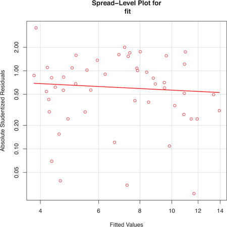
The spreadLevelPlot() function creates a scatter plot of the absolute standardized residuals versus the fitted values, and superimposes a line of best fit. Both functions are demonstrated in listing 8.7.

Listing 8.7. Assessing homoscedasticity

> library(car)
> ncvTest(fit)

Non-constant Variance Score Test
Variance formula: ~ fitted.values
Chisquare=1.7    Df=1     p=0.19

> spreadLevelPlot(fit)

Suggested power transformation:  1.2

The score test is nonsignificant (p = 0.19), suggesting that you’ve met the constant variance assumption. You can also see this in the spread-level plot (figure 8.12). The points form a random horizontal band around a horizontal line of best fit. If you’d violated the assumption, you’d expect to see a nonhorizontal line. The suggested power transformation in listing 8.7 is the suggested power p (Y^p) that would stabilize the nonconstant error variance. For example, if the plot showed a nonhorizontal trend and the suggested power transformation was 0.5, then using rather than Y in the regression equation might lead to a model that satisfies homoscedasticity. If the suggested power was 0, you’d use a log transformation. In the current example, there’s no evidence of heteroscedasticity and the suggested power is close to 1 (no transformation required).

Figure 8.12. Spread-level plot for assessing constant error variance

8.3.3. Global validation of linear model assumption

Finally, let’s examine the gvlma() function in the gvlma package. Written by Pena and Slate (2006), the gvlma() function performs a global validation of linear model assumptions as well as separate evaluations of skewness, kurtosis, and heteroscedasticity. In other words, it provides a single omnibus (go/no go) test of model assumptions. The following listing applies the test to the states data.

Listing 8.8. Global test of linear model assumptions

> library(gvlma)
> gvmodel <- gvlma(fit)
> summary(gvmodel)

ASSESSMENT OF THE LINEAR MODEL ASSUMPTIONS
USING THE GLOBAL TEST ON 4 DEGREES-OF-FREEDOM:
Level of Significance= 0.05

Call:
 gvlma(x=fit)

                   Value p-value                Decision
Global Stat        2.773   0.597 Assumptions acceptable.
Skewness           1.537   0.215 Assumptions acceptable.
Kurtosis           0.638   0.425 Assumptions acceptable.
Link Function      0.115   0.734 Assumptions acceptable.
Heteroscedasticity 0.482   0.487 Assumptions acceptable.

You can see from the printout (the Global Stat line) that the data meet all the statistical assumptions that go with the OLS regression model (p = 0.597). If the decision line had indicated that the assumptions were violated (say, p < 0.05), you’d have had to explore the data using the previous methods discussed in this section to determine which assumptions were the culprit.

8.3.4. Multicollinearity

Before leaving this section on regression diagnostics, let’s focus on a problem that’s not directly related to statistical assumptions but is important in allowing you to interpret multiple regression results.

Imagine you’re conducting a study of grip strength. Your independent variables include date of birth (DOB) and age. You regress grip strength on DOB and age and find a significant overall F test at p < .001. But when you look at the individual regression coefficients for DOB and age, you find that they’re both nonsignificant (that is, there’s no evidence that either is related to grip strength). What happened?

The problem is that DOB and age are perfectly correlated within rounding error. A regression coefficient measures the impact of one predictor variable on the response variable, holding all other predictor variables constant. This amounts to looking at the relationship of grip strength and age, holding age constant. The problem is called multicollinearity. It leads to large confidence intervals for your model parameters and makes the interpretation of individual coefficients difficult.

Multicollinearity can be detected using a statistic called the variance inflation factor (VIF). For any predictor variable, the square root of the VIF indicates the degree to which the confidence interval for that variable’s regression parameter is expanded relative to a model with uncorrelated predictors (hence the name). VIF values are provided by the vif() function in the car package. As a general rule, indicates a multicollinearity problem. The code is provided in the following listing. The results indicate that multicollinearity isn’t a problem with our predictor variables.

Listing 8.9. Evaluating multicollinearity

>library(car)
> vif(fit)

Population Illiteracy     Income      Frost
       1.2        2.2        1.3        2.1

> sqrt(vif(fit)) > 2 # problem?
Population Illiteracy     Income      Frost
     FALSE      FALSE      FALSE      FALSE

8.4. Unusual observations

A comprehensive regression analysis will also include a screening for unusual observations—namely outliers, high-leverage observations, and influential observations. These are data points that warrant further investigation, either because they’re different than other observations in some way, or because they exert a disproportionate amount of influence on the results. Let’s look at each in turn.

8.4.1. Outliers

Outliers are observations that aren’t predicted well by the model. They have either unusually large positive or negative residuals (Y_i - ). Positive residuals indicate that the model is underestimating the response value, while negative residuals indicate an overestimation.

You’ve already seen one way to identify outliers. Points in the Q-Q plot of figure 8.9 that lie outside the confidence band are considered outliers. A rough rule of thumb is that standardized residuals that are larger than 2 or less than –2 are worth attention.

The car package also provides a statistical test for outliers. The outlierTest() function reports the Bonferroni adjusted p-value for the largest absolute studentized residual:

  > library(car)
  > outlierTest(fit)

       rstudent unadjusted p-value  Bonferonni p
Nevada      3.5            0.00095         0.048

Here, you see that Nevada is identified as an outlier (p = 0.048). Note that this function tests the single largest (positive or negative) residual for significance as an outlier. If it isn’t significant, there are no outliers in the dataset. If it is significant, you must delete it and rerun the test to see if others are present.

8.4.2. High leverage points

Observations that have high leverage are outliers with regard to the other predictors. In other words, they have an unusual combination of predictor values. The response value isn’t involved in determining leverage.

Observations with high leverage are identified through the hat statistic. For a given dataset, the average hat value is p/n, where p is the number of parameters estimated in the model (including the intercept) and n is the sample size. Roughly speaking, an observation with a hat value greater than 2 or 3 times the average hat value should be examined. The code that follows plots the hat values:

hat.plot <- function(fit) {
              p <- length(coefficients(fit))
              n <- length(fitted(fit))
              plot(hatvalues(fit), main="Index Plot of Hat Values")
              abline(h=c(2,3)*p/n, col="red", lty=2)
              identify(1:n, hatvalues(fit), names(hatvalues(fit)))
            }
hat.plot(fit)

The resulting graph is shown in figure 8.13.

Figure 8.13. Index plot of hat values for assessing observations with high leverage

Horizontal lines are drawn at 2 and 3 times the average hat value. The locator function places the graph in interactive mode. Clicking on points of interest labels them until the user presses Esc, selects Stop from the graph drop-down menu, or right-clicks on the graph. Here you see that Alaska and California are particularly unusual when it comes to their predictor values. Alaska has a much higher income than other states, while having a lower population and temperature. California has a much higher population than other states, while having a higher income and higher temperature. These states are atypical compared with the other 48 observations.

High leverage observations may or may not be influential observations. That will depend on whether they’re also outliers.

8.4.3. Influential observations

Influential observations are observations that have a disproportionate impact on the values of the model parameters. Imagine finding that your model changes dramatically with the removal of a single observation. It’s this concern that leads you to examine your data for influential points.

There are two methods for identifying influential observations: Cook’s distance, or D statistic and added variable plots. Roughly speaking, Cook’s D values greater than 4/(n-k-1), where n is the sample size and k is the number of predictor variables, indicate influential observations. You can create a Cook’s D plot (figure 8.14) with the following code:

cutoff <- 4/(nrow(states)-length(fit$coefficients)-2)
plot(fit, which=4, cook.levels=cutoff)
abline(h=cutoff, lty=2, col="red")

Figure 8.14. Cook’s D plot for identifying influential observations

The graph identifies Alaska, Hawaii, and Nevada as influential observations. Deleting these states will have a notable impact on the values of the intercept and slopes in the regression model. Note that although it’s useful to cast a wide net when searching for influential observations, I tend to find a cutoff of 1 more generally useful than 4/(n-k-1). Given a criterion of D=1, none of the observations in the dataset would appear to be influential.

Cook’s D plots can help identify influential observations, but they don’t provide information on how these observations affect the model. Added-variable plots can help in this regard. For one response variable and k predictor variables, you’d create k added-variable plots as follows.

For each predictor X_k, plot the residuals from regressing the response variable on the other k-1 predictors versus the residuals from regressing X_k on the other k-1 predictors. Added-variable plots can be created using the avPlots() function in the car package:

library(car)
avPlots(fit, ask=FALSE, onepage=TRUE, id.method="identify")

The resulting graphs are provided in figure 8.15. The graphs are produced one at a time, and users can click on points to identify them. Press Esc, choose Stop from the graph’s menu, or right-click to move on to the next plot. Here, I’ve identified Alaska in the bottom-left plot.

Figure 8.15. Added-variable plots for assessing the impact of influential observations

The straight line in each plot is the actual regression coefficient for that predictor variable. You can see the impact of influential observations by imagining how the line would change if the point representing that observation was deleted. For example, look at the graph of Murder | others versus Income | others in the lower-left corner. You can see that eliminating the point labeled Alaska would move the line in a negative direction. In fact, deleting Alaska changes the regression coefficient for Income from positive (.00006) to negative (–.00085).

You can combine the information from outlier, leverage, and influence plots into one highly informative plot using the influencePlot() function from the car package:

library(car)
influencePlot(fit, id.method="identify", main="Influence Plot",
              sub="Circle size is proportional to Cook's distance")

The resulting plot (figure 8.16) shows that Nevada and Rhode Island are outliers; New York, California, Hawaii, and Washington have high leverage; and Nevada, Alaska, and Hawaii are influential observations.

Figure 8.16. Influence plot. States above +2 or below –2 on the vertical axis are considered outliers. States above 0.2 or 0.3 on the horizontal axis have high leverage (unusual combinations of predictor values). Circle size is proportional to influence. Observations depicted by large circles may have disproportionate influence on the parameters estimates of the model.

8.5. Corrective measures

Having spent the last 20 pages learning about regression diagnostics, you may ask, “What do you do if you identify problems?” There are four approaches to dealing with violations of regression assumptions:

• Deleting observations
• Transforming variables
• Adding or deleting variables
• Using another regression approach

Let’s look at each in turn.

8.5.1. Deleting observations

Deleting outliers can often improve a dataset’s fit to the normality assumption. Influential observations are often deleted as well, because they have an inordinate impact on the results. The largest outlier or influential observation is deleted, and the model is refit. If there are still outliers or influential observations, the process is repeated until an acceptable fit is obtained.

Again, I urge caution when considering the deletion of observations. Sometimes, you can determine that the observation is an outlier because of data errors in recording, or because a protocol wasn’t followed, or because a test subject misunderstood instructions. In these cases, deleting the offending observation seems perfectly reasonable.

In other cases, the unusual observation may be the most interesting thing about the data you’ve collected. Uncovering why an observation differs from the rest can contribute great insight to the topic at hand, and to other topics you might not have thought of. Some of our greatest advances have come from the serendipity of noticing that something doesn’t fit our preconceptions (pardon the hyperbole).

8.5.2. Transforming variables

When models don’t meet the normality, linearity, or homoscedasticity assumptions, transforming one or more variables can often improve or correct the situation. Transformations typically involve replacing a variable Y with Y^λ. Common values of λ and their interpretations are given in table 8.5.

Table 8.5. Common transformations

	–2	–1	–0.5	0	0.5	1	2
Transformation	1/Y2	1/Y	1/	log(Y)		None	Y2

If Y is a proportion, a logit transformation [ln (Y/1-Y)] is often used.

When the model violates the normality assumption, you typically attempt a transformation of the response variable. You can use the powerTransform() function in the car package to generate a maximum-likelihood estimation of the power λ most likely to normalize the variable X^λ. In the next listing, this is applied to the states data.

Listing 8.10. Box–Cox transformation to normality

> library(car)
> summary(powerTransform(states$Murder))

bcPower Transformation to Normality

              Est.Power  Std.Err. Wald Lower Bound Wald Upper Bound
states$Murder       0.6     0.26             0.088              1.1

Likelihood ratio tests about transformation parameters
                      LRT df  pval
LR test, lambda=(0) 5.7  1 0.017
LR test, lambda=(1) 2.1  1 0.145

The results suggest that you can normalize the variable Murder by replacing it with Murder^0.6. Because 0.6 is close to 0.5, you could try a square root transformation to improve the model’s fit to normality. But in this case the hypothesis that λ=1 can’t be rejected (p = 0.145), so there’s no strong evidence that a transformation is actually needed in this case. This is consistent with the results of the Q-Q plot in figure 8.9.

When the assumption of linearity is violated, a transformation of the predictor variables can often help. The boxTidwell() function in the car package can be used to generate maximum-likelihood estimates of predictor powers that can improve linearity. An example of applying the Box–Tidwell transformations to a model that predicts state murder rates from their population and illiteracy rates follows:

> library(car)
> boxTidwell(Murder~Population+Illiteracy,data=states)

           Score Statistic p-value  MLE of lambda
Population           -0.32    0.75           0.87
Illiteracy            0.62    0.54           1.36

The results suggest trying the transformations Population^.87 and Population^1.36 to achieve greater linearity. But the score tests for Population (p = .75) and Illiteracy (p = .54) suggest that neither variable needs to be transformed. Again, these results are consistent with the component plus residual plots in figure 8.11.

Finally, transformations of the response variable can help in situations of heteroscedasticity (nonconstant error variance). You saw in listing 8.7 that the spreadLevelPlot() function in the car package offers a power transformation for improving homoscedasticity. Again, in the case of the states example, the constant error variance assumption is met and no transformation is necessary.

 

 

8.5.3. Adding or deleting variables

Changing the variables in a model will impact the fit of a model. Sometimes, adding an important variable will correct many of the problems that we’ve discussed. Deleting a troublesome variable can do the same thing.

Deleting variables is a particularly important approach for dealing with multicollinearity. If your only goal is to make predictions, then multicollinearity isn’t a problem. But if you want to make interpretations about individual predictor variables, then you must deal with it. The most common approach is to delete one of the variables involved in the multicollinearity (that is, one of the variables with a ). An alternative is to use ridge regression, a variant of multiple regression designed to deal with multicollinearity situations.

8.5.4. Trying a different approach

As you’ve just seen, one approach to dealing with multicollinearity is to fit a different type of model (ridge regression in this case). If there are outliers and/or influential observations, you could fit a robust regression model rather than an OLS regression. If you’ve violated the normality assumption, you can fit a nonparametric regression model. If there’s significant nonlinearity, you can try a nonlinear regression model. If you’ve violated the assumptions of independence of errors, you can fit a model that specifically takes the error structure into account, such as time-series models or multilevel regression models. Finally, you can turn to generalized linear models to fit a wide range of models in situations where the assumptions of OLS regression don’t hold.

We’ll discuss some of these alternative approaches in chapter 13. The decision regarding when to try to improve the fit of an OLS regression model and when to try a different approach, is a complex one. It’s typically based on knowledge of the subject matter and an assessment of which approach will provide the best result.

Speaking of best results, let’s turn now to the problem of deciding which predictor variables to include in our regression model.

8.6. Selecting the “best” regression model

When developing a regression equation, you’re implicitly faced with a selection of many possible models. Should you include all the variables under study, or drop ones that don’t make a significant contribution to prediction? Should you add polynomial and/or interaction terms to improve the fit? The selection of a final regression model always involves a compromise between predictive accuracy (a model that fits the data as well as possible) and parsimony (a simple and replicable model). All things being equal, if you have two models with approximately equal predictive accuracy, you favor the simpler one. This section describes methods for choosing among competing models. The word “best” is in quotation marks, because there’s no single criterion you can use to make the decision. The final decision requires judgment on the part of the investigator. (Think of it as job security.)

8.6.1. Comparing models

You can compare the fit of two nested models using the anova() function in the base installation. A nested model is one whose terms are completely included in the other model. In our states multiple regression model, we found that the regression coefficients for Income and Frost were nonsignificant. You can test whether a model without these two variables predicts as well as one that includes them (see the following listing).

Listing 8.11. Comparing nested models using the anova() function

> fit1 <- lm(Murder ~ Population + Illiteracy + Income + Frost,
          data=states)
> fit2 <- lm(Murder ~ Population + Illiteracy, data=states)
> anova(fit2, fit1)

Analysis of Variance Table

Model 1: Murder ~ Population + Illiteracy
Model 2: Murder ~ Population + Illiteracy + Income + Frost
  Res.Df     RSS  Df     Sum of Sq      F Pr(>F)
1     47 289.246
2     45 289.167  2     0.079 0.0061     0.994

Here, model 1 is nested within model 2. The anova() function provides a simultaneous test that Income and Frost add to linear prediction above and beyond Population and Illiteracy. Because the test is nonsignificant (p = .994), we conclude that they don’t add to the linear prediction and we’re justified in dropping them from our model.

The Akaike Information Criterion (AIC) provides another method for comparing models. The index takes into account a model’s statistical fit and the number of parameters needed to achieve this fit. Models with smaller AIC values—indicating adequate fit with fewer parameters—are preferred. The criterion is provided by the AIC() function (see the following listing).

Listing 8.12. Comparing models with the AIC

> fit1 <- lm(Murder ~ Population + Illiteracy + Income + Frost,
          data=states)
> fit2 <- lm(Murder ~ Population + Illiteracy, data=states)
> AIC(fit1,fit2)

     df      AIC
fit1  6 241.6429
fit2  4 237.6565

The AIC values suggest that the model without Income and Frost is the better model. Note that although the ANOVA approach requires nested models, the AIC approach doesn’t.

Comparing two models is relatively straightforward, but what do you do when there are four, or ten, or a hundred possible models to consider? That’s the topic of the next section.

8.6.2. Variable selection

Two popular approaches to selecting a final set of predictor variables from a larger pool of candidate variables are stepwise methods and all-subsets regression.

Stepwise Regression

In stepwise selection, variables are added to or deleted from a model one at a time, until some stopping criterion is reached. For example, in forward stepwise regression you add predictor variables to the model one at a time, stopping when the addition of variables would no longer improve the model. In backward stepwise regression, you start with a model that includes all predictor variables, and then delete them one at a time until removing variables would degrade the quality of the model. In stepwise stepwise regression (usually called stepwise to avoid sounding silly), you combine the forward and backward stepwise approaches. Variables are entered one at a time, but at each step, the variables in the model are reevaluated, and those that don’t contribute to the model are deleted. A predictor variable may be added to, and deleted from, a model several times before a final solution is reached.

The implementation of stepwise regression methods vary by the criteria used to enter or remove variables. The stepAIC() function in the MASS package performs stepwise model selection (forward, backward, stepwise) using an exact AIC criterion. In the next listing, we apply backward stepwise regression to the multiple regression problem.

Listing 8.13. Backward stepwise selection

> library(MASS)
> fit1 <- lm(Murder ~ Population + Illiteracy + Income + Frost,
          data=states)
> stepAIC(fit, direction="backward")

Start:  AIC=97.75
Murder ~ Population + Illiteracy + Income + Frost

             Df  Sum of Sq    RSS    AIC
- Frost       1       0.02 289.19  95.75
- Income      1       0.06 289.22  95.76
<none>                     289.17  97.75
- Population  1      39.24 328.41 102.11
- Illiteracy  1     144.26 433.43 115.99

Step:  AIC=95.75
Murder ~ Population + Illiteracy + Income

             Df  Sum of Sq    RSS    AIC
- Income      1       0.06 289.25  93.76
<none>                     289.19  95.75
- Population  1      43.66 332.85 100.78
- Illiteracy  1     236.20 525.38 123.61

Step:  AIC=93.76
Murder ~ Population + Illiteracy

             Df  Sum of Sq    RSS    AIC
<none>                     289.25  93.76
- Population  1      48.52 337.76  99.52
- Illiteracy  1     299.65 588.89 127.31

Call:
lm(formula=Murder ~ Population + Illiteracy, data=states)

Coefficients:
(Intercept)   Population    Illiteracy
  1.6515497    0.0002242     4.0807366

You start with all four predictors in the model. For each step, the AIC column provides the model AIC resulting from the deletion of the variable listed in that row. The AIC value for <none> is the model AIC if no variables are removed. In the first step, Frost is removed, decreasing the AIC from 97.75 to 95.75. In the second step, Income is removed, decreasing the AIC to 93.76. Deleting any more variables would increase the AIC, so the process stops.

Stepwise regression is controversial. Although it may find a good model, there’s no guarantee that it will find the best model. This is because not every possible model is evaluated. An approach that attempts to overcome this limitation is all subsets regression.

All Subsets Regression

In all subsets regression, every possible model is inspected. The analyst can choose to have all possible results displayed, or ask for the nbest models of each subset size (one predictor, two predictors, etc.). For example, if nbest=2, the two best one-predictor models are displayed, followed by the two best two-predictor models, followed by the two best three-predictor models, up to a model with all predictors.

All subsets regression is performed using the regsubsets() function from the leaps package. You can choose R-squared, Adjusted R-squared, or Mallows Cp statistic as your criterion for reporting “best” models.

As you’ve seen, R-squared is the amount of variance accounted for in the response variable by the predictors variables. Adjusted R-squared is similar, but takes into account the number of parameters in the model. R-squared always increases with the addition of predictors. When the number of predictors is large compared to the sample size, this can lead to significant overfitting. The Adjusted R-squared is an attempt to provide a more honest estimate of the population R-squared—one that’s less likely to take advantage of chance variation in the data. The Mallows Cp statistic is also used as a stopping rule in stepwise regression. It has been widely suggested that a good model is one in which the Cp statistic is close to the number of model parameters (including the intercept).

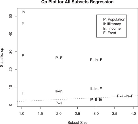
In listing 8.14, we’ll apply all subsets regression to the states data. The results can be plotted with either the plot() function in the leaps package or the subsets() function in the car package. An example of the former is provided in figure 8.17, and an example of the latter is given in figure 8.18.

Figure 8.17. Best four models for each subset size based on Adjusted R-square

Figure 8.18. Best four models for each subset size based on the Mallows Cp statistic

Listing 8.14. All subsets regression

library(leaps)
leaps <-regsubsets(Murder ~ Population + Illiteracy + Income +
  Frost, data=states, nbest=4)
plot(leaps, scale="adjr2")

library(car)
subsets(leaps, statistic="cp",
  main="Cp Plot for All Subsets Regression")
abline(1,1,lty=2,col="red")

Figure 8.17 can be confusing to read. Looking at the first row (starting at the bottom), you can see that a model with the intercept and Income has an adjusted R-square of 0.33. A model with the intercept and Population has an adjusted R-square of 0.1. Jumping to the 12th row, you see that a model with the intercept, Population, Illiteracy, and Income has an adjusted R-square of 0.54, whereas one with the intercept, Population, and Illiteracy alone has an adjusted R-square of 0.55. Here you see that a model with fewer predictors has a larger adjusted R-square (something that can’t happen with an unadjusted R-square). The graph suggests that the two-predictor model (Population and Illiteracy) is the best.

In figure 8.18, you see the best four models for each subset size based on the Mallows Cp statistic. Better models will fall close to a line with intercept 1 and slope 1. The plot suggests that you consider a two-predictor model with Population and Illiteracy; a three-predictor model with Population, Illiteracy, and Frost, or Population, Illiteracy and Income (they overlap on the graph and are hard to read); or a four-predictor model with Population, Illiteracy, Income, and Frost. You can reject the other possible models.

In most instances, all subsets regression is preferable to stepwise regression, because more models are considered. However, when the number of predictors is large, the procedure can require significant computing time. In general, automated variable selection methods should be seen as an aid rather than a directing force in model selection. A well-fitting model that doesn’t make sense doesn’t help you. Ultimately, it’s your knowledge of the subject matter that should guide you.

8.7. Taking the analysis further

We’ll end our discussion of regression by considering methods for assessing model generalizability and predictor relative importance.

8.7.1. Cross-validation

In the previous section, we examined methods for selecting the variables to include in a regression equation. When description is your primary goal, the selection and interpretation of a regression model signals the end of your labor. But when your goal is prediction, you can justifiably ask, “How well will this equation perform in the real world?”

By definition, regression techniques obtain model parameters that are optimal for a given set of data. In OLS regression, the model parameters are selected to minimize the sum of squared errors of prediction (residuals), and conversely, maximize the amount of variance accounted for in the response variable (R-squared). Because the equation has been optimized for the given set of data, it won’t perform as well with a new set of data.

We began this chapter with an example involving a research physiologist who wanted to predict the number of calories an individual will burn from the duration and intensity of their exercise, age, gender, and BMI. If you fit an OLS regression equation to this data, you’ll obtain model parameters that uniquely maximize the R-squared for this particular set of observations. But our researcher wants to use this equation to predict the calories burned by individuals in general, not only those in the original study. You know that the equation won’t perform as well with a new sample of observations, but how much will you lose? Cross-validation is a useful method for evaluating the generalizability of a regression equation.

In cross-validation, a portion of the data is selected as the training sample and a portion is selected as the hold-out sample. A regression equation is developed on the training sample, and then applied to the hold-out sample. Because the hold-out sample wasn’t involved in the selection of the model parameters, the performance on this sample is a more accurate estimate of the operating characteristics of the model with new data.

In k-fold cross-validation, the sample is divided into k subsamples. Each of the k subsamples serves as a hold-out group and the combined observations from the remaining k-1 subsamples serves as the training group. The performance for the k prediction equations applied to the k hold-out samples are recorded and then averaged. (When k equals n, the total number of observations, this approach is called jackknifing.)

You can perform k-fold cross-validation using the crossval() function in the bootstrap package. The following listing provides a function (called shrinkage()) for cross-validating a model’s R-square statistic using k-fold cross-validation.

Listing 8.15. Function for k-fold cross-validated R-square

shrinkage <- function(fit, k=10){
  require(bootstrap)

  theta.fit <- function(x,y){lsfit(x,y)}
  theta.predict <- function(fit,x){cbind(1,x)%*%fit$coef}

  x <- fit$model[,2:ncol(fit$model)]
  y <- fit$model[,1]

  results <- crossval(x, y, theta.fit, theta.predict, ngroup=k)
  r2 <- cor(y, fit$fitted.values)^2
  r2cv <- cor(y, results$cv.fit)^2
  cat("Original R-square =", r2, "
")
  cat(k, "Fold Cross-Validated R-square =", r2cv, "
")
  cat("Change =", r2-r2cv, "
")
  }

Using this listing you define your functions, create a matrix of predictor and predicted values, get the raw R-squared, and get the cross-validated R-squared. (Chapter 12 covers bootstrapping in detail.)

The shrinkage() function is then used to perform a 10-fold cross-validation with the states data, using a model with all four predictor variables:

> fit <- lm(Murder ~ Population + Income + Illiteracy + Frost, data=states)
> shrinkage(fit)

Original R-square=0.567
10 Fold Cross-Validated R-square=0.4481
Change=0.1188

You can see that the R-square based on our sample (0.567) is overly optimistic. A better estimate of the amount of variance in murder rates our model will account for with new data is the cross-validated R-square (0.448). (Note that observations are assigned to the k groups randomly, so you will get a slightly different result each time you execute the shrinkage() function.)

You could use cross-validation in variable selection by choosing a model that demonstrates better generalizability. For example, a model with two predictors (Population and Illiteracy) shows less R-square shrinkage (.03 versus .12) than the full model:

> fit2 <- lm(Murder~Population+Illiteracy,data=states)
> shrinkage(fit2)

Original R-square=0.5668327
10 Fold Cross-Validated R-square=0.5346871
Change=0.03214554

This may make the two-predictor model a more attractive alternative.

All other things being equal, a regression equation that’s based on a larger training sample and one that’s more representative of the population of interest will cross-validate better. You’ll get less R-squared shrinkage and make more accurate predictions.

8.7.2. Relative importance

Up to this point in the chapter, we’ve been asking, “Which variables are useful for predicting the outcome?” But often your real interest is in the question, “Which variables are most important in predicting the outcome?” You implicitly want to rank-order the predictors in terms of relative importance. There may be practical grounds for asking the second question. For example, if you could rank-order leadership practices by their relative importance for organizational success, you could help managers focus on the behaviors they most need to develop.

If predictor variables were uncorrelated, this would be a simple task. You would rank-order the predictor variables by their correlation with the response variable. In most cases, though, the predictors are correlated with each other, and this complicates the task significantly.

There have been many attempts to develop a means for assessing the relative importance of predictors. The simplest has been to compare standardized regression coefficients. Standardized regression coefficients describe the expected change in the response variable (expressed in standard deviation units) for a standard deviation change in a predictor variable, holding the other predictor variables constant. You can obtain the standardized regression coefficients in R by standardizing each of the variables in your dataset to a mean of 0 and standard deviation of 1 using the scale() function, before submitting the dataset to a regression analysis. (Note that because the scale() function returns a matrix and the lm() function requires a data frame, you convert between the two in an intermediate step.) The code and results for our multiple regression problem are shown here:

> zstates <- as.data.frame(scale(states))
> zfit <- lm(Murder~Population + Income + Illiteracy + Frost, data=zstates)
> coef(zfit)

(Intercept)  Population      Income  Illiteracy       Frost
 -9.406e-17   2.705e-01   1.072e-02   6.840e-01   8.185e-03

Here you see that a one standard deviation increase in illiteracy rate yields a 0.68 standard deviation increase in murder rate, when controlling for population, income, and temperature. Using standardized regression coefficients as our guide, Illiteracy is the most important predictor and Frost is the least.

There have been many other attempts at quantifying relative importance. Relative importance can be thought of as the contribution each predictor makes to R-square, both alone and in combination with other predictors. Several possible approaches to relative importance are captured in the relaimpo package written by Ulrike Grömping (http://prof.beuth-hochschule.de/groemping/relaimpo/).

A new method called relative weights shows significant promise. The method closely approximates the average increase in R-square obtained by adding a predictor variable across all possible submodels (Johnson, 2004; Johnson and Lebreton, 2004; LeBreton and Tonidandel, 2008). A function for generating relative weights is provided in the next listing.

Listing 8.16. relweights() function for calculating relative importance of predictors

relweights <- function(fit,...){
  R <- cor(fit$model)
  nvar <- ncol(R)
  rxx <- R[2:nvar, 2:nvar]
  rxy <- R[2:nvar, 1]
  svd <- eigen(rxx)
  evec <- svd$vectors
  ev <- svd$values
  delta <- diag(sqrt(ev))
  lambda <- evec %*% delta %*% t(evec)
  lambdasq <- lambda ^ 2
  beta <- solve(lambda) %*% rxy
  rsquare <- colSums(beta ^ 2)
  rawwgt <- lambdasq %*% beta ^ 2
  import <- (rawwgt / rsquare) * 100
  lbls <- names(fit$model[2:nvar])
  rownames(import) <- lbls
  colnames(import) <- "Weights"
  barplot(t(import),names.arg=lbls,
     ylab="% of R-Square",
     xlab="Predictor Variables",
     main="Relative Importance of Predictor Variables",
     sub=paste("R-Square=", round(rsquare, digits=3)),
     ...)
return(import)
}

 

Note

The code in listing 8.16 is adapted from an SPSS program generously provided by Dr. Johnson. See Johnson (2000, Multivariate Behavioral Research, 35, 1–19) for an explanation of how the relative weights are derived.

 

In listing 8.17 the relweights() function is applied to the states data with murder rate predicted by the population, illiteracy, income, and temperature.

You can see from figure 8.19 that the total amount of variance accounted for by the model (R-square=0.567) has been divided among the predictor variables. Illiteracy accounts for 59 percent of the R-square, Frost accounts for 20.79 percent, and so forth. Based on the method of relative weights, Illiteracy has the greatest relative importance, followed by Frost, Population, and Income, in that order.

Figure 8.19. Bar plot of relative weights for the states multiple regression problem

Listing 8.17. Applying the relweights() function

> fit <- lm(Murder ~ Population + Illiteracy + Income + Frost, data=states)
> relweights(fit, col="lightgrey")

            Weights
Population    14.72
Illiteracy    59.00
Income         5.49
Frost         20.79

Relative importance measures (and in particular, the method of relative weights) have wide applicability. They come much closer to our intuitive conception of relative importance than standardized regression coefficients do, and I expect to see their use increase dramatically in coming years.

8.8. Summary

Regression analysis is a term that covers a broad range of methodologies in statistics. You’ve seen that it’s a highly interactive approach that involves fitting models, assessing their fit to statistical assumptions, modifying both the data and the models, and refitting to arrive at a final result. In many ways, this final result is based on art and skill as much as science.

This has been a long chapter, because regression analysis is a process with many parts. We’ve discussed fitting OLS regression models, using regression diagnostics to assess the data’s fit to statistical assumptions, and methods for modifying the data to meet these assumptions more closely. We looked at ways of selecting a final regression model from many possible models, and you learned how to evaluate its likely performance on new samples of data. Finally, we tackled the thorny problem of variable importance: identifying which variables are the most important for predicting an outcome.

In each of the examples in this chapter, the predictor variables have been quantitative. However, there are no restrictions against using categorical variables as predictors as well. Using categorical predictors such as gender, treatment type, or manufacturing process allows you to examine group differences on a response or outcome variable. This is the focus of our next chapter.