
Chapter 12. Resampling statistics and bootstrapping
In chapters 7, 8, and 9, we reviewed statistical methods that test hypotheses and estimate confidence intervals for population parameters by assuming that the observed data is sampled from a normal distribution or some other well-known theoretical distribution. But there will be many cases in which this assumption is unwarranted. Statistical approaches based on randomization and resampling can be used in cases where the data is sampled from unknown or mixed distributions, where sample sizes are small, where outliers are a problem, or where devising an appropriate test based on a theoretical distribution is too complex and mathematically intractable.
In this chapter, we’ll explore two broad statistical approaches that use randomization: permutation tests and bootstrapping. Historically, these methods were only available to experienced programmers and expert statisticians. Contributed packages in R now make them readily available to a wider audience of data analysts.
We’ll also revisit problems that were initially analyzed using traditional methods (for example, t-tests, chi-square tests, ANOVA, regression) and see how they can be approached using these robust, computer-intensive methods. To get the most out of section 12.2, be sure to read chapter 7 first. Chapters 8 and 9 serve as prerequisites for section 12.3. Other sections can be read on their own.
12.1. Permutation tests
Permutation tests, also called randomization or re-randomization tests, have been around for decades, but it took the advent of high-speed computers to make them practically available.
To understand the logic of a permutation test, consider the following hypothetical problem. Ten subjects have been randomly assigned to one of two treatment conditions (A or B) and an outcome variable (score) has been recorded. The results of the experiment are presented in table 12.1.
Table 12.1. Hypothetical two-group problem
|
Treatment A |
Treatment B |
|---|---|
| 40 | 57 |
| 57 | 64 |
| 45 | 55 |
| 55 | 62 |
| 58 | 65 |
The data are also displayed in the strip chart in figure 12.1. Is there enough evidence to conclude that the treatments differ in their impact?
Figure 12.1. Strip chart of the hypothetical treatment data in table 12.1

In a parametric approach, you might assume that the data are sampled from normal populations with equal variances and apply a two-tailed independent groups t-test. The null hypothesis is that the population mean for treatment A is equal to the population mean for treatment B. You’d calculate a t-statistic from the data and compare it to the theoretical distribution. If the observed t-statistic is sufficiently extreme, say outside the middle 95 percent of values in the theoretical distribution, you’d reject the null hypothesis and declare that the population means for the two groups are unequal at the 0.05 level of significance.
A permutation test takes a different approach. If the two treatments are truly equivalent, the label (Treatment A or Treatment B) assigned to an observed score is arbitrary. To test for differences between the two treatments, we could follow these steps:
1. Calculate the observed t-statistic, as in the parametric approach; call this t0.
2. Place all 10 scores in a single group.
3. Randomly assign five scores to Treatment A and five scores to Treatment B.
4. Calculate and record the new observed t-statistic.
5. Repeat steps 3–4 for every possible way of assigning five scores to Treatment A and five scores to Treatment B. There are 252 such possible arrangements.
6. Arrange the 252 t-statistics in ascending order. This is the empirical distribution, based on (or conditioned on) the sample data.
7. If t0 falls outside the middle 95 percent of the empirical distribution, reject the null hypothesis that the population means for the two treatment groups are equal at the 0.05 level of significance.
Notice that the same t-statistic is calculated in both the permutation and parametric approaches. But instead of comparing the statistic to a theoretical distribution in order to determine if it was extreme enough to reject the null hypothesis, it’s compared to an empirical distribution created from permutations of the observed data. This logic can be extended to most classical statistical tests and linear models.
In the previous example, the empirical distribution was based on all possible permutations of the data. In such cases, the permutation test is called an “exact” test. As the sample sizes increase, the time required to form all possible permutations can become prohibitive. In such cases, you can use Monte Carlo simulation to sample from all possible permutations. Doing so provides an approximate test.
If you’re uncomfortable assuming that the data is normally distributed, concerned about the impact of outliers, or feel that the dataset is too small for standard parametric approaches, a permutation test provides an excellent alternative.
R has some of the most comprehensive and sophisticated packages for performing permutation tests currently available. The remainder of this section focuses on two contributed packages: the coin package and the lmPerm package. Be sure to install them before first use:
install.packages(c("coin","lmPerm"))
The coin package provides a comprehensive framework for permutation tests applied to independence problems, whereas the lmPerm package provides permutation tests for ANOVA and regression designs. We’ll consider each in turn, and end the section with a quick review of other permutation packages available in R.
Before moving on, it’s important to remember that permutation tests use pseudorandom numbers to sample from all possible permutations (when performing an approximate test). Therefore, the results will change each time the test is performed. Setting the random number seed in R allows you to fix the random numbers generated. This is particularly useful when you want to share your examples with others, because results will always be the same if the calls are made with the same seed. Setting the random number seed to 1234 (that is, set.seed(1234)) will allow you to replicate the results presented in this chapter.
12.2. Permutation test with the coin package
The coin package provides a general framework for applying permutation tests to independence problems. With this package, we can answer such questions as
- Are responses independent of group assignment?
- Are two numeric variables independent?
- Are two categorical variables independent?
Using convenience functions provided in the package (see table 12.2), we can perform permutation test equivalents for most of the traditional statistical tests covered in chapter 7.
Table 12.2. coin functions providing permutation test alternatives to traditional tests
|
Test |
coin function |
|---|---|
| Two- and K-sample permutation test | oneway_test(y ~ A) |
| Two- and K-sample permutation test with a stratification (blocking) factor | oneway_test(y ~ A | C) |
| Wilcoxon–Mann–Whitney rank sum test | wilcox_test(y ~ A) |
| Kruskal–Wallis test | kruskal_test(y ~ A) |
| Person’s chi-square test | chisq_test(A ~ B) |
| Cochran–Mantel–Haenszel test | cmh_test(A ~ B | C) |
| Linear-by-linear association test | lbl_test(D ~ E) |
| Spearman’s test | spearman_test(y ~ x) |
| Friedman test | friedman_test(y ~ A | C) |
| Wilcoxon–Signed–Rank test | wilcoxsign_test(y1 ~ y2) |
| In the coin function column, y and x are numeric variables, A and B are categorical factors, C is a categorical blocking variable, D and E are ordered factors, and y1 and y2 are matched numeric variables. | |
Each of the functions listed in table 12.2 take the form
function_name( formula, data, distribution= )
where
- formula describes the relationship among variables to be tested. Examples are given in the table.
- data identifies a data frame.
- distribution specifies how the empirical distribution under the null hypothesis should be derived. Possible values are exact, asymptotic, and approximate.
If distribution=“exact”, the distribution under the null hypothesis is computed exactly (that is, from all possible permutations). The distribution can also be approximated by its asymptotic distribution (distribution=“asymptotic”) or via Monte Carlo resampling (distribution=“approximate(B=#)”), where # indicates the number of replications used to approximate the exact distribution. At present, distribution=“exact” is only available for two-sample problems.
Note
In the coin package, categorical variables and ordinal variables must be coded as factors and ordered factors, respectively. Additionally, the data must be stored in a data frame.
In the remainder of this section, we’ll apply several of the permutation tests described in table 12.2 to problems from previous chapters. This will allow you to compare the results with more traditional parametric and nonparametric approaches. We’ll end this discussion of the coin package by considering advanced extensions.
12.2.1. Independent two-sample and k-sample tests
To begin, compare an independent samples t-test with a one-way exact test applied to the hypothetical data in table 12.2. The results are given in the following listing.
Listing 12.1. t-test versus one-way permutation test for the hypothetical data
> library(coin)
> score <- c(40, 57, 45, 55, 58, 57, 64, 55, 62, 65)
> treatment <- factor(c(rep("A",5), rep("B",5)))
> mydata <- data.frame(treatment, score)
> t.test(score~treatment, data=mydata, var.equal=TRUE)

        Two Sample t-test

data:  score by treatment
t = -2.3, df = 8, p-value = 0.04705
alternative hypothesis: true difference in means is not equal to 0
95 percent confidence interval:
 -19.04  -0.16
sample estimates:
mean in group A mean in group B
             51              61

> oneway_test(score~treatment, data=mydata, distribution="exact")

        Exact 2-Sample Permutation Test

data:  score by treatment (A, B)
Z = -1.9, p-value = 0.07143
alternative hypothesis: true mu is not equal to 0
The traditional t-test indicates a significant group difference (p < .05), whereas the exact test doesn’t (p > 0.072). With only 10 observations, l’d be more inclined to trust the results of the permutation test and attempt to collect more data before reaching a final conclusion.
Next, consider the Wilcoxon–Mann–Whitney U test. In chapter 7, we examined the difference in the probability of imprisonment in Southern versus non-Southern US states using the wilcox.test() function. Using an exact Wilcoxon rank sum test, we’d get
> library(MASS)
> UScrime <- transform(UScrime, So = factor(So))
> wilcox_test(Prob ~ So, data=UScrime, distribution="exact")

        Exact Wilcoxon Mann-Whitney Rank Sum Test

data:  Prob by So (0, 1)
Z = -3.7, p-value = 8.488e-05
alternative hypothesis: true mu is not equal to 0
suggesting that incarceration is more likely in Southern states. Note that in the previous code, the numeric variable So was transformed into a factor. This is because the coin package requires that all categorical variables be coded as factors. Additionally, the astute reader may have noted that these results agree exactly with the results of the wilcox.test() in chapter 7. This is because the wilcox.test() also computes an exact distribution by default.
Finally, consider a k-sample test. In chapter 9, we used a one-way ANOVA to evaluate the impact of five drug regimens on cholesterol reduction in a sample of 50 patients. An approximate k-sample permutation test can be performed instead, using this code:
> library(multcomp)
> set.seed(1234)
> oneway_test(response~trt, data=cholesterol,
  distribution=approximate(B=9999))

        Approximative K-Sample Permutation Test

data:  response by
         trt (1time, 2times, 4times, drugD, drugE)
maxT = 4.7623, p-value < 2.2e-16
Here, the reference distribution is based on 9,999 permutations of the data. The random number seed was set so that your results would be the same as mine. There’s clearly a difference in response among patients in the various groups.
12.2.2. Independence in contingency tables
We can use permutation tests to assess the independence of two categorical variables using either the chisq_test() or the cmh_test() function. The latter function is used when the data is stratified on a third categorical variable. If both variables are ordinal, we can use the lbl_test() function to test for a linear trend.
In chapter 7, we applied a chi-square test to assess the relationship between Arthritis treatment and improvement. Treatment had two levels (Placebo, Treated), and Improved had three levels (None, Some, Marked). The Improved variable was encoded as an ordered factor.
If you want to perform a permutation version of the chi-square test, you could use the following code:
> library(coin)
> library(vcd)
> Arthritis <- transform(Arthritis,
  Improved=as.factor(as.numeric(Improved)))
> set.seed(1234)
> chisq_test(Treatment~Improved, data=Arthritis,
             distribution=approximate(B=9999))

                Approximative Pearson's Chi-Squared Test

data:  Treatment by Improved (1, 2, 3)
chi-squared = 13.055, p-value = 0.0018
This gives you an approximate chi-square test based on 9,999 replications. You might ask why you transformed the variable Improved from an ordered factor to a categorical factor. (Good question!) If you’d left it an ordered factor, coin() would have generated a linear x linear trend test instead of a chi-square test. Although a trend test would be a good choice in this situation, keeping it a chi-square test allows you to compare the results with those reported in chapter 7.
12.2.3. Independence between numeric variables
The spearman_test() function provides a permutation test of the independence of two numeric variables. In chapter 7, we examined the correlation between illiteracy rates and murder rates for US states. You can test the association via permutation, using the following code:
> states <- as.data.frame(state.x77)
> set.seed(1234)
> spearman_test(Illiteracy~Murder, data=states,
                distribution=approximate(B=9999))

        Approximative Spearman Correlation Test

data:  Illiteracy by Murder
Z = 4.7065, p-value < 2.2e-16
alternative hypothesis: true mu is not equal to 0
Based on an approximate permutation test with 9,999 replications, the hypothesis of independence can be rejected. Note that state.x77 is a matrix. It had to be converted into a data frame for use in the coin package.
12.2.4. Dependent two-sample and k-sample tests
Dependent sample tests are used when observations in different groups have been matched, or when repeated measures are used. For permutation tests with two paired groups, the wilcoxsign_test() function can be used. For more than two groups, use the friedman_test() function.
In chapter 7, we compared the unemployment rate for urban males age 14–24 (U1) with urban males age 35–39 (U2). Because the two variables are reported for each of the 50 US states, you have a two-dependent groups design (state is the matching variable). We can use an exact Wilcoxon Signed Rank Test to see if unemployment rates for the two age groups are equal:
> library(coin)
> library(MASS)
> wilcoxsign_test(U1~U2, data=UScrime, distribution="exact")

        Exact Wilcoxon-Signed-Rank Test

data:  y by x (neg, pos)
         stratified by block
Z = 5.9691, p-value = 1.421e-14
alternative hypothesis: true mu is not equal to 0
Based on the results, you’d conclude that the unemployment rates differ.
12.2.5. Going further
The coin package provides a general framework for testing that one group of variables is independent of a second group of variables (with optional stratification on a blocking variable) against arbitrary alternatives, via approximate permutation tests. In particular, the independence_test() function allows the user to approach most traditional tests from a permutation perspective, and to create new and novel statistical tests for situations not covered by traditional methods. This flexibility comes at a price: a high level of statistical knowledge is required to use the function appropriately. See the vignettes that accompany the package (accessed via vignette(“coin”)) for further details.
In the next section, you’ll learn about the lmPerm package. This package provides a permutation approach to linear models, including regression and analysis of variance.
12.3. Permutation tests with the lmPerm package
The lmPerm package provides support for a permutation approach to linear models. In particular, the lmp() and aovp() functions are the lm() and aov() functions modified to perform permutation tests rather than normal theory tests.
The parameters within the lmp() and aovp() functions are similar to those in the lm() and aov() functions, with the addition of a perm= parameter. The perm= option can take on the values “Exact”, “Prob”, or “SPR”. Exact produces an exact test, based on all possible permutations. Prob samples from all possible permutations. Sampling continues until the estimated standard deviation falls below 0.1 of the estimated p-value. The stopping rule is controlled by an optional Ca parameter. Finally, SPR uses a sequential probability ratio test to decide when to stop sampling. Note that if the number of observations is greater than 10, perm=“Exact” will automatically default to perm=“Prob”; exact tests are only available for small problems.
To see how this works, we’ll apply a permutation approach to simple regression, polynomial regression, multiple regression, one-way analysis of variance, one-way analysis of covariance, and a two-way factorial design.
12.3.1. Simple and polynomial regression
In chapter 8, we used linear regression to study the relationship between weight and height for a group of 15 women. Using lmp() instead of lm() generates the permutation test results shown in the following listing.
Listing 12.2. Permutation tests for simple linear regression
> library(lmPerm)
> set.seed(1234)
> fit <- lmp(weight~height, data=women, perm="Prob")
[1] "Settings:  unique SS : numeric variables centered"
> summary(fit)

Call:
lmp(formula = weight ~ height, data = women, perm = "Prob")

Residuals:
   Min     1Q Median     3Q    Max
-1.733 -1.133 -0.383  0.742  3.117

Coefficients:
       Estimate Iter Pr(Prob)
height     3.45 5000   <2e-16 ***
---
Signif. codes:  0 '***' 0.001 '**' 0.01 '*' 0.05 '.' 0.1 ' ' 1

Residual standard error: 1.5 on 13 degrees of freedom
Multiple R-Squared: 0.991,      Adjusted R-squared: 0.99
F-statistic: 1.43e+03 on 1 and 13 DF,  p-value: 1.09e-14
To fit a quadratic equation, you could use the code in this next listing.
Listing 12.3. Permutation tests for polynomial regression
> library(lmPerm)
> set.seed(1234)
> fit <- lmp(weight~height + I(height^2), data=women, perm="Prob")
[1] "Settings:  unique SS : numeric variables centered"
> summary(fit)

Call:
lmp(formula = weight ~ height + I(height^2), data = women, perm = "Prob")

Residuals:
    Min      1Q  Median      3Q     Max
-0.5094 -0.2961 -0.0094  0.2862  0.5971

Coefficients:
            Estimate Iter Pr(Prob)
height       -7.3483 5000    <2e-16 ***
I(height^2)   0.0831 5000    <2e-16 ***
---
Signif. codes:  0 '***' 0.001 '**' 0.01 '*' 0.05 '.' 0.1 ' ' 1

Residual standard error: 0.38 on 12 degrees of freedom
Multiple R-Squared: 0.999,      Adjusted R-squared: 0.999
F-statistic: 1.14e+04 on 2 and 12 DF,  p-value: <2e-16
As you can see, it’s a simple matter to test these regressions using permutation tests and requires little change in the underlying code. The output is also similar to that produced by the lm() function. Note that an Iter column is added indicating how many iterations were required to reach the stopping rule.
12.3.2. Multiple regression
In chapter 8, multiple regression was used to predict the murder rate from population, illiteracy, income, and frost for 50 US states. Applying the lmp() function to this problem, results in the following output.
Listing 12.4. Permutation tests for multiple regression
> library(lmPerm)
> set.seed(1234)
> states <- as.data.frame(state.x77)
> fit <- lmp(Murder~Population + Illiteracy+Income+Frost,
             data=states, perm="Prob")
[1] "Settings:  unique SS : numeric variables centered"
> summary(fit)

Call:
lmp(formula = Murder ~ Population + Illiteracy + Income + Frost,
    data = states, perm = "Prob")

Residuals:
     Min       1Q   Median       3Q      Max
-4.79597 -1.64946 -0.08112  1.48150  7.62104

Coefficients:
            Estimate Iter Pr(Prob)
Population 2.237e-04   51   1.0000
Illiteracy 4.143e+00 5000   0.0004 ***
Income     6.442e-05   51   1.0000
Frost      5.813e-04   51   0.8627
---
Signif. codes:  0 '***' 0.001 '**' 0.01 '*' 0.05 '. ' 0.1 ' ' 1

Residual standard error: 2.535 on 45 degrees of freedom
Multiple R-Squared: 0.567,      Adjusted R-squared: 0.5285
F-statistic: 14.73 on 4 and 45 DF,  p-value: 9.133e-08
Looking back to chapter 8, both Population and Illiteracy are significant (p < 0.05) when normal theory is used. Based on the permutation tests, the Population variable is no longer significant. When the two approaches don’t agree, you should look at your data more carefully. It may be that the assumption of normality is untenable or that outliers are present.
12.3.3. One-way ANOVA and ANCOVA
Each of the analysis of variance designs discussed in chapter 9 can be performed via permutation tests. First, let’s look at the one-way ANOVA problem considered in sections 9.1 on the impact of treatment regimens on cholesterol reduction. The code and results are given in the next listing.
Listing 12.5. Permutation test for One-Way ANOVA
> library(lmPerm)
> library(multcomp)
> set.seed(1234)
> fit <- aovp(response~trt, data=cholesterol, perm="Prob")
[1] "Settings:  unique SS "
> summary(fit)
Component 1 :
            Df R Sum Sq R Mean Sq Iter  Pr(Prob)
trt          4  1351.37    337.84 5000 < 2.2e-16 ***
Residuals   45   468.75     10.42
---
Signif. codes:  0 '***' 0.001 '**' 0.01 '*' 0.05 '. ' 0.1 ' ' 1
The results suggest that the treatment effects are not all equal.
This second example in this section applies a permutation test to a one-way analysis of covariance. The problem is from chapter 9, where you investigated the impact of four drug doses on the litter weights of rats, controlling for gestation times. The next listing shows the permutation test and results.
Listing 12.6. Permutation test for one-way ANCOVA
> library(lmPerm)
> set.seed(1234)
> fit <- aovp(weight ~ gesttime + dose, data=litter, perm="Prob")
[1] "Settings:  unique SS : numeric variables centered"
> summary(fit)
Component 1 :
            Df R Sum Sq R Mean Sq Iter Pr(Prob)
gesttime     1   161.49   161.493 5000   0.0006 ***
dose         3   137.12    45.708 5000   0.0392 *
Residuals   69  1151.27    16.685
---
Signif. codes:  0 '***' 0.001 '**' 0.01 '*' 0.05 '.' 0.1 ' ' 1
Based on the p-values, the four drug doses do not equally impact litter weights, controlling for gestation time.
12.3.4. Two-way ANOVA
We’ll end this section by applying permutation tests to a factorial design. In chapter 9, we examined the impact of vitamin C on the tooth growth in guinea pigs. The two manipulated factors were dose (three levels) and delivery method (two levels). Ten guinea pigs were placed in each treatment combination, resulting in a balanced 3 x 2 factorial design. The permutation tests are provided in the next listing.
Listing 12.7. Permutation test for two-way ANOVA
> library(lmPerm)
> set.seed(1234)
> fit <- aovp(len~supp*dose, data=ToothGrowth, perm="Prob")
[1] "Settings:  unique SS : numeric variables centered"
> summary(fit)
Component 1 :
            Df R Sum Sq  R Mean Sq Iter Pr(Prob)
supp         1   205.35     205.35 5000  < 2e-16 ***
dose         1  2224.30    2224.30 5000  < 2e-16 ***
supp:dose    1    88.92      88.92 2032  0.04724 *
Residuals   56   933.63      16.67
---
Signif. codes:  0 '***' 0.001 '**' 0.01 '*' 0.05 '.' 0.1 ' ' 1
At the .05 level of significance, all three effects are statistically different from zero. At the .01 level, only the main effects are significant.
It’s important to note that when aovp() is applied to ANOVA designs, it defaults to unique sums of squares (also called SAS Type III sums of squares). Each effect is adjusted for every other effect. The default for parametric ANOVA designs in R is sequential sums of squares (SAS Type I sums of squares). Each effect is adjusted for those that appear earlier in the model. For balanced designs, the two approaches will agree, but for unbalanced designs with unequal numbers of observations per cell, they won’t. The greater the imbalance, the greater the disagreement. If desired, specifying seqs=TRUE in the aovp() function will produce sequential sums of squares. For more on Type I and Type III sums of squares, see chapter 9, section 9.2.
12.4. Additional comments on permutation tests
R offers other permutation packages besides coin and lmPerm. The perm package provides some of the same functionality provided by the coin package and can act as an independent validation of that package. The corrperm package provides permutation tests of correlations with repeated measures. The logregperm package offers a permutation test for logistic regression. Perhaps most importantly, the glmperm package extends permutation tests to generalized linear models. Generalized linear models are described in the next chapter.
Permutation tests provide a powerful alternative to tests that rely on a knowledge of the underlying sampling distribution. In each of the permutation tests described, we were able to test statistical hypotheses without recourse to the normal, t, F, or chi-square distributions.
You may have noticed how closely the results of the tests based on normal theory agreed with the results of the permutation approach in previous sections. The data in these problems were well behaved and the agreement between methods is a testament to how well normal theory methods work in such cases.
Where permutation tests really shine are in cases where the data is clearly non-normal (for example, highly skewed), outliers are present, samples sizes are small, or no parametric tests exist. However, if the original sample is a poor representation of the population of interest, no test, including permutation tests, will improve the inferences generated.
Permutation tests are primarily useful for generating p-values that can be used to test null hypotheses. They can help answer the question, “Does an effect exist?” It’s more difficult to use permutation methods to obtain confidence intervals and estimates of measurement precision. Fortunately, this is an area in which bootstrapping excels.
12.5. Bootstrapping
Bootstrapping generates an empirical distribution of a test statistic or set of test statistics, by repeated random sampling with replacement, from the original sample. It allows you to generate confidence intervals and test statistical hypotheses without having to assume a specific underlying theoretical distribution.
It’s easiest to demonstrate the logic of bootstrapping with an example. Say that you want to calculate the 95 percent confidence interval for a sample mean. Your sample has 10 observations, a sample mean of 40, and a sample standard deviation of 5. If you’re willing to assume that the sampling distribution of the mean is normally distributed, the (1-α/2)% confidence interval can be calculated using
![]()
where t is the upper 1-α/2 critical value for at distribution with n-1 degrees of freedom. For a 95 percent confidence interval, you have 40 – 2.262(5/3.163) < µ < 40 + 2.262(5/3.162) or 36.424 < µ < 43.577. You’d expect 95 percent of confidence intervals created in this way to surround the true population mean.
But what if you aren’t willing to assume that the sampling distribution of the mean is normally distributed? You could use a bootstrapping approach instead:
- Randomly select 10 observations from the sample, with replacement after each selection. Some observations may be selected more than once, and some may not be selected at all.
- Calculate and record the sample mean.
- Repeat steps 1 and 2 a thousand times.
- Order the 1,000 sample means from smallest to largest.
- Find the sample means representing the 2.5th and 97.5th percentiles. In this case, it’s the 25th number from the bottom and top. These are your 95 percent confidence limits.
In the present case, where the sample mean is likely to be normally distributed, you gain little from the bootstrap approach. Yet there are many cases where the bootstrap approach is advantageous. What if you wanted confidence intervals for the sample median, or the difference between two sample medians? There are no simple normal theory formulas here, and bootstrapping is the approach of choice. If the underlying distributions are unknown, if outliers are a problem, if sample sizes are small, or if parametric approaches don’t exist, bootstrapping can often provide a useful method of generating confidence intervals and testing hypotheses.
12.6. Bootstrapping with the boot package
The boot package provides extensive facilities for bootstrapping and related resampling methods. You can bootstrap a single statistic (for example, a median), or a vector of statistics (for example, a set of regression coefficients). Be sure to download and install the boot package before first use:
install.packages("boot")
The bootstrapping process will seem complicated, but once you review the examples it should make sense.
In general, bootstrapping involves three main steps:
1. Write a function that returns the statistic or statistics of interest. If there is a single statistic (for example, a median), the function should return a number. If there is a set of statistics (for example, a set of regression coefficients), the function should return a vector.
2. Process this function through the boot() function in order to generate R bootstrap replications of the statistic(s).
3. Use the boot.ci() function to obtain confidence intervals for the statistic(s) generated in step 2.
Now to the specifics.
The main bootstrapping function is boot(). The boot() function has the format
bootobject <- boot(data=, statistic=, R=, ...)
The parameters are described in table 12.3.
Table 12.3. Parameters of the boot() function
|
Parameter |
Description |
|---|---|
| data | A vector, matrix, or data frame. |
| statistic | A function that produces the k statistics to be bootstrapped (k=1 if bootstrapping a single statistic). |
| The function should include an indices parameter that the boot() function can use to select cases for each replication (see examples in the text). | |
| R | Number of bootstrap replicates. |
| ... | Additional parameters to be passed to the function that is used to produce statistic(s) of interest. |
The boot() function calls the statistic function R times. Each time, it generates a set of random indices, with replacement, from the integers 1:nrow(data). These indices are used within the statistic function to select a sample. The statistics are calculated on the sample and the results are accumulated in the bootobject. The bootobject structure is described in table 12.4.
Table 12.4. Elements of the object returned by the boot() function
|
Element |
Description |
|---|---|
| t0 | The observed values of k statistics applied to the original data |
| t | An R × k matrix where each row is a bootstrap replicate of the k statistics |
You can access these elements as bootobject$t0 and bootobject$t.
Once you generate the bootstrap samples, you can use print() and plot() to examine the results. If the results look reasonable, you can use the boot.ci() function to obtain confidence intervals for the statistic(s). The format is
boot.ci(bootobject, conf=, type= )
The parameters are given in table 12.5.
Table 12.5. Parameters of the boot.ci() function
|
Parameter |
Description |
|---|---|
| bootobject | The object returned by the boot() function. |
| conf | The desired confidence interval (default: conf=0.95). |
| type | The type of confidence interval returned. Possible values are “norm”, “basic”, “stud”, “perc”, “bca”, and “all” (default: type="all"). |
The type parameter specifies the method for obtaining the confidence limits. The perc method (percentile) was demonstrated in the sample mean example. The bca provides an interval that makes simple adjustments for bias. I find bca preferable in most circumstances. See Mooney and Duval (1993) for an introduction to these methods.
In the remaining sections, we’ll look at bootstrapping a single statistic and a vector of statistics.
12.6.1. Bootstrapping a single statistic
The mtcars dataset contains information on 32 automobiles reported in the 1974 Motor Trend magazine. Suppose you’re using multiple regression to predict miles per gallon from a car’s weight (lb/1,000) and engine displacement (cu. in.). In addition to the standard regression statistics, you’d like to obtain a 95 percent confidence interval for the R-squared value (the percent of variance in the response variable explained by the predictors). The confidence interval can be obtained using nonparametric bootstrapping.
The first task is to write a function for obtaining the R-squared value:
rsq <- function(formula, data, indices) {
         d <- data[indices,]
         fit <- lm(formula, data=d)
         return(summary(fit)$r.square)

}
The function returns the R-square value from a regression. The d <- data[indices,] statement is required for boot() to be able to select samples.
You can then draw a large number of bootstrap replications (say, 1,000) with the following code:
library(boot)
set.seed(1234)
results <- boot(data=mtcars, statistic=rsq,
                R=1000, formula=mpg~wt+disp)
The boot object can be printed using
> print(results)

ORDINARY NONPARAMETRIC BOOTSTRAP


Call:
boot(data = mtcars, statistic = rsq, R = 1000, formula = mpg ~
    wt + disp)


Bootstrap Statistics :
     original     bias    std. error
t1* 0.7809306 0.01333670  0.05068926
and plotted using plot(results). The resulting graph is shown in figure 12.2.
Figure 12.2. Distribution of bootstrapped R-squared values
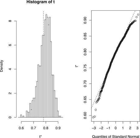
In figure 12.2, you can see that the distribution of bootstrapped R-squared values isn’t normally distributed. A 95 percent confidence interval for the R-squared values can be obtained using
> boot.ci(results, type=c("perc", "bca"))
BOOTSTRAP CONFIDENCE INTERVAL CALCULATIONS
Based on 1000 bootstrap replicates

CALL :
boot.ci(boot.out = results, type = c("perc", "bca"))

Intervals :
Level     Percentile            BCa
95%   ( 0.6838,  0.8833 )   ( 0.6344,  0.8549 )
Calculations and Intervals on Original Scale
Some BCa intervals may be unstable
You can see from this example that different approaches to generating the confidence intervals can lead to different intervals. In this case the bias adjusted interval is moderately different from the percentile method. In either case, the null hypothesis H0: R-square = 0, would be rejected, because zero is outside the confidence limits.
In this section, we estimated the confidence limits of a single statistic. In the next section, we’ll estimate confidence intervals for several statistics.
12.6.2. Bootstrapping several statistics
In the previous example, bootstrapping was used to estimate the confidence interval for a single statistic (R-squared). Continuing the example, let’s obtain the 95 percent confidence intervals for a vector of statistics. Specifically, let’s get confidence intervals for the three model regression coefficients (intercept, car weight, and engine displacement).
First, create a function that returns the vector of regression coefficients:
bs <- function(formula, data, indices) {
        d <- data[indices,]
        fit <- lm(formula, data=d)
        return(coef(fit))
}
Then use this function to bootstrap 1,000 replications:
library(boot)
set.seed(1234)
results <- boot(data=mtcars, statistic=bs,
                R=1000, formula=mpg~wt+disp)
> print(results)
ORDINARY NONPARAMETRIC BOOTSTRAP
Call:
boot(data = mtcars, statistic = bs, R = 1000, formula = mpg ~
    wt + disp)

Bootstrap Statistics :
    original   bias    std. error
t1*  34.9606  0.137873     2.48576
t2*  -3.3508 -0.053904     1.17043
t3*  -0.0177 -0.000121     0.00879
When bootstrapping multiple statistics, add an index parameter to the plot() and boot.ci() functions to indicate which column of bootobject$t to analyze. In this example, index 1 refers to the intercept, index 2 is car weight, and index 3 is the engine displacement. To plot the results for car weight, use
plot(results, index=2)
The graph is given in figure 12.3.
Figure 12.3. Distribution of bootstrapping regression coefficients for car weight

To get the 95 percent confidence intervals for car weight and engine displacement, use
> boot.ci(results, type="bca", index=2)
BOOTSTRAP CONFIDENCE INTERVAL CALCULATIONS
Based on 1000 bootstrap replicates

CALL :
boot.ci(boot.out = results, type = "bca", index = 2)
Intervals :
Level       BCa
95%   (-5.66, -1.19 )
Calculations and Intervals on Original Scale

> boot.ci(results, type="bca", index=3)

BOOTSTRAP CONFIDENCE INTERVAL CALCULATIONS
Based on 1000 bootstrap replicates

CALL :
boot.ci(boot.out = results, type = "bca", index = 3)

Intervals :
Level       BCa
95%   (-0.0331,  0.0010 )
Calculations and Intervals on Original Scale
Note
In the previous example, we resampled the entire sample of data each time. If we assume that the predictor variables have fixed levels (typical in planned experiments), we’d do better to only resample residual terms. See Mooney and Duval (1993, pp. 16–17) for a simple explanation and algorithm.
Before we leave bootstrapping, it’s worth addressing two questions that come up often:
- How large does the original sample need to be?
- How many replications are needed?
There’s no simple answer to the first question. Some say that an original sample size of 20–30 is sufficient for good results, as long as the sample is representative of the population. Random sampling from the population of interest is the most trusted method for assuring the original sample’s representativeness. With regard to the second question, I find that 1,000 replications are more than adequate in most cases. Computer power is cheap and you can always increase the number of replications if desired.
There are many helpful sources of information on permutation tests and bootstrapping. An excellent starting place is an online article by Yu (2003). Good (2006) provides a comprehensive overview of resampling in general and includes R code. A good, accessible introduction to the bootstrap is provided by Mooney and Duval (1993). The definitive source on bootstrapping is Efron and Tibshirani (1998). Finally, there are a number of great online resources, including Simon (1997), Canty (2002), Shah (2005), and Fox (2002).
12.7. Summary
In this chapter, we introduced a set of computer-intensive methods based on randomization and resampling that allow you to test hypotheses and form confidence intervals without reference to a known theoretical distribution. They’re particularly valuable when your data comes from unknown population distributions, when there are serious outliers, when your sample sizes are small, and when there are no existing parametric methods to answer the hypotheses of interest.
The methods in this chapter are particularly exciting because they provide an avenue for answering questions when your standard data assumptions are clearly untenable, or when you have no other idea how to approach the problem. Permutation tests and bootstrapping aren’t panaceas, though. They can’t turn bad data into good data. If your original samples aren’t representative of the population of interest, or are too small to accurately reflect it, then these techniques won’t help.
In the next chapter, we’ll consider data models for variables that follow known, but not necessarily normal, distributions.