CHAPTER 12

A Multiple-Equations Approach to Long-Term Forecasting

Short-term forecasting is not the only important element of decision making. Several important decisions consider the longer-term economic outlook.¹ For instance, a firm's budget, investment, and employment decisions often incorporate the economic outlook for the next five to seven years. Long-term forecasting of key economic and financial variables, therefore, plays a crucial role in public and private sector decision making. This chapter presents procedures useful to develop models for long-term economic and business forecasting, which differ in several ways from the steps of short-run forecasting.²

When building forecasting models for a longer time period, an analyst should keep a few important points in mind. First, the chances of significant changes in the economic environment are very high. Forecasting the value of the Standard & Poor's (S&P) 500 index a few years out is not easy because there is a high probability of significant changes in the model for equity returns. In January 2008, for example, the U.S. economy was in recession and the S&P 500 index was in bearish territory. If an analyst was trying to make a forecast for the S&P 500 index two years ahead, he or she would struggle with the assumptions. If the recession ended in 2008 and was followed by a strong recovery, the S&P 500 index would have quickly turned bullish. However, that was not the case.³ So longer-term forecasting is associated with higher uncertainty when compared to a shorter-term forecast horizon.

Second, many macroeconomic variables behave differently during different phases of the business cycle. The average business cycle duration, defined as trough to trough since World War II, is around 70 months. The U.S. unemployment rate tends to rise during recessions and fall during expansions. An analyst interested in forecasting the unemployment rate for the next six to eight years would always need to consider business cycle movements.

Third, analysts need to consider policy changes. The two major political parties have very different tax and spending preferences. Elections thus may also affect the accuracy of long-term forecasting. Hence, the possibility of a structural change due to internal policy change or external shocks is higher during long-term forecasting compared to short-term prediction.

The last factor analysts need to think about is that the variables and model selection procedures are different for long-term forecasting from those for short-term forecasting. As mentioned in Chapters 10 and 11, in short-term forecasting, the predictors and final model specification are selected based on simulated out-of-sample root mean square error (RMSE), where the model with the smallest simulated out-of-sample RMSE is chosen. In long-term forecasting, large-scale macroeconometric models that utilize hundreds of variables and dozens of regression equations are all built on the basis of an economic theory.⁴ There are at least two major reasons for this approach. The first reason is that the chance of a significant change in the behavior of a macroeconomic variable is higher in the long run, which can influence other sectors of the economy. For instance, the boom and subsequent bust in the U.S. housing sector was one of the major causes of the Great Recession and financial crisis of 2007 to 2009. Changes in the behavior of the housing sector therefore influenced changes in many other sectors of the U.S. economy. Forecasters often do not know ahead of time which sector of the economy will lead to changes in other sectors. Therefore, it is important to include as much information as possible in the long-term forecasting model. Typically, a forecaster wants to include key predictors representing major sectors of the economy in the model.

The second reason to rely on theory instead of statistical measures to create a long-term forecasting model is that most economic and financial data series do not have a long history—an essential element to calculate simulated out-of-sample RMSE. For instance, in Chapter 11, we mentioned that we finalize short-term forecasting models based on the simulated out-of-sample RMSE. That is, we calculate simulated out-of-sample RMSEs for different model specifications and select the model that produces the smallest RMSE. In the case of long-term forecasting, due to a lack of a longer history of the dataset, it would be difficult to estimate simulated out-of-sample RMSE for different models and then compare those with each other to select the best model based on RMSE.⁵

Once an analyst selects the variables for the long-term forecast model, the next step is to estimate the model. There are two major categories of estimation methods: unconditional forecasting models and conditional forecasting models.

The unconditional forecasting approach utilizes Bayesian vector autoregression (BVAR) models. The BVAR approach is termed unconditional because it does not require future values of the right-hand-side variables to generate out-of-sample forecasts for target variables (this is covered in depth in the next section of this chapter). The conditional forecasting approach extends the single-equation approach (explained in Chapter 10) into a multiple equation system. The out-of-sample forecasts of the target variables are conditioned on the future values of the right-hand-side variables.

While both the conditional and unconditional long-term forecasting approaches identify variables of interest with the help of economic and financial theory, the unconditional approach forecasts based on the current and past values of the dataset while the conditional approach develops different scenarios for the target variables based on conditional future values of the right-hand-side variables. For instance, later in this chapter we look at what happens to U.S. economic growth if oil prices suddenly rise to $150 per barrel from $95 per barrel. This chapter discusses both the unconditional and conditional forecasting approaches and provides SAS codes helpful in generating these forecasts.

THE UNCONDITIONAL LONG-TERM FORECASTING: THE BVAR MODEL

In this section we explore the unconditional long-term forecasting approach, utilizing BVAR models. Before we discuss the BVAR approach, we look at the limitations of large-scale macro models, which were the major tools for long-term forecasting before the introduction of VAR/BVAR. For long-term forecasting, the traditional Keynesian models known as large-scale macro models seem to have been the natural tools from the 1950s to the 1970s.⁶ In the late 1970s, however, a few prominent economists criticized the theoretical foundation of these models.⁷ They thought that the traditional models consisting of dozens, if not hundreds, of econometric regressions were usually too large for the individual analyst to use effectively. They also recognized that forecasting with the traditional models requires the future values of the models' exogenous variables, which are often hard to predict. In addition, in practice, it is difficult to determine which variables are endogenous and which are exogenous. This is also known as the identification problem. (See Sims [1980] for more detail.) For these reasons, traditional largescale macro models may not be easy to build in practice.

Sims (1980) provided a new framework for macroeconomic forecasting known as vector autoregressions (VAR). A VAR is an n-equation, n-variable model in which each variable is a linear function of its own lagged values, plus the lagged values of the other n−1 variables. In a VAR there are no exogenous variables. In other words, all variables are treated equally and the n variables are endogenous; future values of these variables can easily be forecasted due to the VAR approach's dynamic setup. The VAR approach has proven to be a powerful and reliable forecasting method in everyday use.⁸ However, there is a technical problem despite its success. Macroeconomic time series usually have short sample sizes (e.g., quarterly gross domestic product [GDP] or monthly unemployment rate) while the number of VAR parameters increases rapidly with the increase in the number of variables and lags. This many parameters creates an over-fitting problem that leads to a good in-sample fit but poor out-of-sample forecasting performance. To avoid the over-fitting problem, a typical VAR has to be relatively small. Litterman (1980) presented the BVAR approach to address this problem.⁹ As mentioned in Chapter 11, Litterman's method imposes prior restrictions, also known as Minnesota Prior, on the VAR parameters. The prior allows the inclusion of a larger number of variables and their lags in the BVAR model compared to the traditional VAR model. Litterman (1986) showed that his approach is as accurate, on average, as those utilized by the best-known commercial forecasting services (DRI, Chase, and Wharton at that time).¹⁰

Variable selection is an important aspect of the BVAR (and VAR) forecasting approach. The variables should represent key sectors of the economy, but, at the same time, the analyst should not include too many variables, as that would create an over-fitting problem.

For example, if the goal is to create a BAVR model of the U.S. economy, the analyst would be able to create an accurate forecast using an eight-variable BVAR model. The variables are: real GDP, 10-year Treasury yields, industrial production, unemployment rate, consumer price index, S&P 500 index, trade-weighted dollar, and the Commodity Futures Price index. Essentially we try to include variables from major sectors of the economy. In this case, real GDP (GDP) represents the broad economy, while 10-year Treasury yields (Ten_year) capture the effects of interest rates and borrowing costs on the economy. The unemployment rate (RUC) is a good labor market indicator, and CPI is a proxy for the inflation rate. Industrial production (IP) represents the production side of the economy, and the S&P 500 index (SP500) is utilized to represent the financial sector and the services sector, as major companies are closely related with the S&P 500 index. The U.S. economy is an open economy in which the exchange rate plays a key role in international trade. Trade-weighted index (Dollar) is included to capture the exchange rate effect on the economy. Commodities prices also affect the inflation rate and overall economy; that is why we include the CRB index (CRB) in the BVAR model.

Once an analyst decides to employ the BVAR approach for long-term forecasting and selects the variables for the model, the next step is to utilize SAS to estimate the model and generate forecasts. SAS code S12.1 estimates the eight-variables BVAR model.

PROC VARMAX offers the BVAR option. The data file bvar_data contains all eight variables. After the SAS keyword Model, we listed the variables of interests. The lag order (denoted by p) is 6, meaning that up to six lags of each variable are included in the BVAR model. The prior values lambda=.4 and theta=.3 are used.¹¹ The SAS keyword ID instructs SAS to utilize the variable name date as ID, and the interval is quarterly. The term output is another SAS keyword that generates and saves out-of-sample forecasts for all eight variables. The output is saved in a data file named forecast_bvar, and lead=8 shows that eight quarters ahead is to be forecasted. We employ a quarterly dataset for the 1986:Q1 = 2013:Q1 period.

The forecasts based on SAS code S12.1 are presented in Table 12.1. The model predicted a GDP growth rate around 3 percent over the next eight quarters, peaking at 3.38 percent in 2014:Q3. The CPI shows an inflation rate of below 2 percent for the 2013–2014 periods. Both the industrial production and S&P 500 show strong growth rates. The dollar index is weakening, and the CRB index shows a moderate growth rate compared to historical standards. The 10-year Treasury yield stays below 2 percent, and the unemployment rate has a decreasing trend. Overall, the BVAR model predicts a moderate growth scenario for the U.S. economy.

For a visual look, the actual GDP growth, GDP forecasts, and the upper and lower forecast limits for a 95 percent interval are plotted in Figure 12.1.¹² The forecast seems accurate because the actual values and the forecasted values stay mostly within the forecast band, although, in Q4-2008 the actual GDP value crossed the lower limit of the forecast. One reason this may have happened is because the depth of the Great Recession was a surprise to many economists and analysts. However, the model did correctly predict the direction. Overall, the chart suggests that the BVAR model's forecasting performance is reliable.

THE BVAR MODEL WITH HOUSING STARTS

Given the importance of the housing sector on the performance of the U.S. economy, we look at another BVAR model, which includes housing starts data to capture housing sector activity. In this model we did not include the trade-weighted dollar. Therefore, the BVAR model still contains eight variables. SAS code S12.2 estimates the BVAR model with housing starts (HS_YoY), using the same lag and prior values as in S12.1.

TABLE 12.1 Forecasts Based on the Eight-Variable BVAR Model

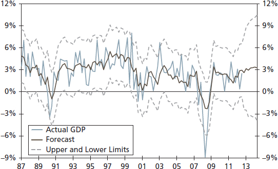
FIGURE 12.1 GDP Forecasts Based on the Eight-Variable BVAR Model

Table 12.2 reports forecasts based on code S12.2. The forecasts point toward relatively stronger growth rates for the U.S. economy compared to the one presented in Table 12.1. One major reason for this relatively stronger forecast is that the housing sector was a major cause of the Great Recession. Without a solid recovery in the housing sector, the overall economy may not experience a fast and strong recovery. The BVAR model predicts stronger growth rates for housing starts (a solid recovery), boosting the overall economy's growth rates.

Figure 12.2 plots actual GDP growth, the forecast with housing starts and the 95 percent interval based on the BVAR model with housing starts. The forecasts seem relatively accurate as the actual and forecast figures stay mostly within the forecast band.

Figure 12.3 shows actual GDP growth along with the forecast based on the original eight-variable BVAR model and the modified model with housing starts.

In summary, an analyst can generate forecasts for key economic and financial variables using the BVAR model. The SAS codes we used in S12.1 and S12.2 can be used to forecast any variable by replacing the listed variables with others of interest.

THE MODEL WITHOUT OIL PRICE SHOCK

The BVAR model's use of past and current values to forecast defines the approach as unconditional. However, sometimes it may be essential for decision makers to predict the future paths of key economic and financial variables under different policy environments or in the face of an external shock, such as an oil price shock.

TABLE 12.2 Forecasts Based on the Modified Model with Housing Starts

FIGURE 12.2 GDP Forecasts Based on the Modified Model with Housing Starts

FIGURE 12.3 GDP Forecasts Based on the Original and Modified BVAR Model

What would happen to the economy if oil prices suddenly increased? The price for West Texas Intermediate crude oil (WTI) peaked at $133.88 per barrel on June 2008, a 98.4 percent increase from $67.49 per barrel just one year earlier. This swift price increase shocked consumers and squeezed their wallets as retail gasoline prices hit $4.00 per gallon for the first time. Such a shock to consumers and on their confidence and their willingness to spend could have large negative effects on economic activity. For this reason, decision makers might want to forecast economic growth under various scenarios, specifically oil price shocks. In this case study, we utilize the conditional forecasting approach and generate forecasts conditioned on a scenario with and without an oil price shock.

As mentioned previously, building a large-scale macro model to forecast the outcome of economic shocks is difficult. A more practical approach is to develop a small-scale multiple-equation model to generate conditional forecasts. For our case study, we create an eight-equation, eight-variable model. We utilize the same variables used in the BVAR model in the previous section. Because these variables represent major sectors of the U.S. economy, they can help build a small but effective macro model.

In this approach we build eight equations: one for each variable (equation 12.1). Each equation includes a lag of the dependent variable along with seven other variables as right-hand-side variables. The WTI crude oil price, our measure for oil prices, is also included in each equation as an exogenous variable.

Essentially, we are following the VAR logic and treating all variables as equal by building an equation for each variable; this implies that all of the variables are interconnected and dependent on each other. This solves the identification problem. The variable for oil prices, WTI, is left as the only exogenous variable that is not given its own model.

A Small-Scale Macro Model: Equation 12.1

In equation 12.1, GDP is the real GDP growth rate, Ten_Yr is the 10-year Treasury yield, UR is the unemployment rate, CPI is our proxy for inflation and IP stands for industrial production, the S&P500 index is denoted by SP500, the trade-weighted dollar is dollar, commodity prices are indicated by CRB, and WTI is our measure for oil prices. ε1 to ε8 are error terms of the model, and ao to h9 are the parameters to be estimated. SAS code S12.3 is employed to estimate the small-scale macro model described in Equation 12.1. The dataset covers the 1986:Q1 to 2013:Q1 time period for estimation, and conditional forecasts are generated for the 2013:Q2 to 2014:Q4 period.

As mentioned in Chapter 10, PROC MODEL is a flexible procedure to estimate multiple equation models, also known as large- and small-scale macro models. The SAS keyword fit instructs SAS to consider listed variables (in this case the eight variables) as dependent variables. The solve option will generate forecasts for each of the eight variables. The output is saved in the data file named Forecast_WTI.

As stated earlier, the forecasts are conditioned on the future values of exogenous variables and, in the present case, WTI. Note that there may be more than one exogenous variable. In the first example, our base case, we assume that there is no price shock. However, even though we forecast no shock, we still need to generate future values for our model. We decide to use the average price of the last five years (2008–2012) of $86.32 per barrel as our forecasted values. That is, we believe the price of oil will remain near its average over the forecast horizon. The forecasts are reported in Table 12.3. The GDP growth rates stay around 1.6 to 1.9 percent with the unemployment rate remaining at elevated levels. Overall, the forecast postulates a slower growth scenario.

TABLE 12.3 Forecasts Conditioned on the Average WTI Price Model: Without an Oil Price Shock Scenario

FIGURE 12.4 GDP Forecasts Conditioned on the Average WTI Prices: Without an Oil Price Shock Scenario

In Figure 12.4 we plot the actual and forecasted GDP growth rates. The forecast appears to be consistent with movements in the actual GDP growth rates, although the decline in GDP growth during 2008 was much larger than forecasted.

THE MODEL WITH OIL PRICE SHOCK

In this section, we create long-term forecasts under the assumption that the price of oil rises. We used the five-year average price for the predicted future values of a barrel of WTI in the previous section; here we increase the price of WTI to $150 per barrel over the 2013:Q2–2014:Q4 time period. This strong jump in price represents the oil price shock. We use the same SAS code, S12.3, that was utilized in the previous example to model this scenario, with the only difference being the future values of WTI. The forecasts are presented in Table 12.4 and are very different from those reported in Table 12.3. When predicting an upward jump in oil prices, the GDP growth rates drop into negative territory in 2013:Q3 and remain negative for the forecast horizon. Moreover, the unemployment rate increases and peaks in 2014:Q4 at 9.63 percent. Industrial production and the S&P 500 index also suggest negative growth rates for 2014. We can conclude that a rise in oil prices can have negative, and significant, effects on the economy.

Figure 12.5 shows the actual and forecasted GDP growth rates in the case of an oil price shock. The forecast indicates a recession beginning in 2013.

TABLE 12.4 Forecasts Based on the Higher WTI Price Model: The Oil Price Shock Scenario

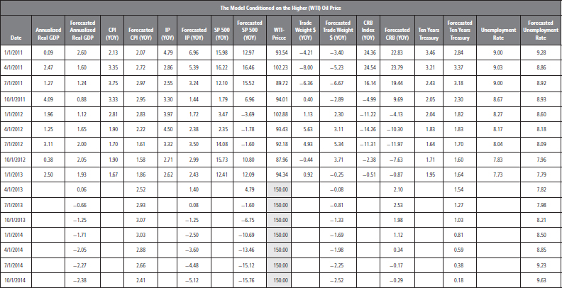
FIGURE 12.5 GDP Forecasts Conditioned on Higher WTI Prices: The Oil Price Shock Scenario

In summary, the conditional forecasting approach is very useful when analyzing different policy implications and external shocks. To show the risk to forecasts due to uncertainty, it is wise to predict different scenarios and the likely growth paths for the variables of interest. We presented only one scenario, but the basic idea to build a small-scale macro model and generate forecasts for different scenarios can be replicated for any policy change or external shock.

SUMMARY

Long-term forecasting approaches are an important element in decision making. In the case of unconditional forecasting, the BVAR approach is suggested. The BVAR approach utilizes past and current values of the dataset and generates forecasts for the target variables. In the conditional forecasting approach, a practical option is to build a small-scale macro model that can be utilized to generate forecasts for the target variables.

Both approaches are useful to public and private decision making. The benefit of unconditional forecasting is that it provides neutral forecasts and lets the data speak for itself. Conditional forecasting, in contrast, is an essential tool to analyze the impact of a policy change and/or of an external shock on the economy.

An analyst should become familiar with both approaches and utilize the SAS codes provided in the chapter for long-term forecasting.