CHAPTER 13

The Risks of Model-Based Forecasting: Modeling, Assessing, and Remodeling

This chapter highlights risks and challenges to model-based forecasting and also provides guidelines to minimize the forecast errors stemming from those risks. The nature of forecast risks differs depending on the duration of the forecast. We divide these risks into two broad categories: (1) risks related to short-term forecasting and (2) risks related to long-term forecasting.

In short-term forecasting, the chance of a permanent shift in the behavior of a series is low, but sometimes factors, such as a hurricane or a work-related strike, can affect the outcome. Including those factors in a model is difficult due to their unexpected and temporary nature. That said, adjustments can be made to the model's forecast to reduce forecast error.

For long-run forecasting, the event's nature tends to be permanent, and the chance of significant changes, or structural breaks, is very high. For instance, trying to forecast the path of home prices during the housing boom of the late 1990s through the mid-2000s would have been very difficult. From January 1997 to December 2005, the Standard & Poor's (S&P)/Case-Shiller House Price Index (HPI) followed a strong increasing trend—a trend that many analysts speculated would continue for the foreseeable future. However, the index peaked in April 2006, and a strong downward trend followed. The break in the prior trend was unexpected and therefore difficult to forecast. How could the analyst prepare for such unexpected changes in long-run data? One possible solution would be to generate scenario-based forecasts of the S&P/Case-Shiller HPI to include the possibility of a decline in prices even though prices may not have fallen in the recent past.

In this chapter, we also discuss the financial crisis of 2007 to 2009 and its effect on economic forecasts and suggest that, in some instances, even a forecaster cannot predict a financial panic. A better way to analyze likely scenarios is to closely monitor the patterns and changes of variables and to incorporate those patterns into a model's output.

In the last section of this chapter, we summarize overall thoughts about model-based forecasting and suggest three phases to model-based forecasting: (1) modeling, (2) assessing, and (3) remodeling. These three interconnected phases are essential for both short-term and long-term forecasting.

RISKS TO SHORT-TERM FORECASTING: THERE IS NO MAGIC BULLET

When devising short-term forecasting—forecasting outcomes one to two months in advance—there is little incidence of significant changes in the economic environment, and therefore little chance of a structural shift in the data. For instance, a one-month-ahead forecast of the S&P 500 index or a firm's forecast for the next quarter's earnings would not likely be subject to a significant structural change in the model. Sometimes short-term forecasting may face significant changes—for example, a natural disaster like Hurricane Katrina that shocks the data instantly. There are some occasions, however, when an analyst finds it necessary to adjust the forecast to reduce error. This may or may not include rebuilding the model. In this section, we provide suggestions as to when it is necessary to rebuild the model.

Forecasting economic and financial series is like sailing a boat. The analyst should constantly monitor the performance of the model and make adjustments to the (financial and economic) winds and currents. Many analysts, however, try to find the best forecasting model at the time and then continue to use it even if the environment has changed. Unfortunately, models often break down over time and become less accurate at predicting future movements.

Monitoring a model's performance need not be difficult. Here are some useful evaluating techniques. If the forecast misses the direction of the actual value for three consecutive months, then the analyst should revise the model.¹ Moreover, periodically the analyst can compare the model's performance to others in the field. For example, the analyst can compare the model to Bloomberg's consensus using real-time out-of-sample root mean squared error (RMSE) and directional accuracy criteria. If a model has a higher RMSE and lower directional accuracy compared to the Bloomberg consensus, then the model should be reconstructed. If a model needs to be revised, the analyst can follow the procedure described in Chapter 11.²

After the Great Recession of 2007 to 2009, many economic and financial data series were turned upside down, causing most forecasting models to become ineffective. We will run through an example using the Bayesian vector autoregression (BVAR) nonfarm payrolls model. Prior to the Great Recession, the analyst's model for nonfarm payrolls could have been very accurate. As markets turned and businesses shed jobs by the millions, the model broke down completely. For instance, the real-time, out-of-sample, one-month-forward RMSE of the original nonfarm payrolls model from October 2006 to February 2008 was 51,000, beating the Bloomberg consensus RMSE of 54,000. However, once the economy began to fall apart, and job growth began to contract dramatically, the analyst likely noticed his or her forecast missing the direction of growth (continuing to foresee growth in payrolls when in reality jobs were declining). At this time, if the analyst rebuilt the model, he or she would have achieved a new RMSE of 75,000 for January 2009 to August 2010. If the analyst continued to use the old model, the new RMSE would have been 110,000—significantly worse than the rebuilt model. We suggest that real-time, short-term forecasting involves three phases: (1) building new models, (2) continuously monitoring the forecasting performance of these models, and (3) constructing new models when these models break down. In an age of ever-changing economies, one model specification will not remain accurate forever. Even the best model specification will need to be revised.

One important thing to note is that the nature of the event shocking the economic data will have different influences on the accuracy of the model. Some events are temporary and affect the accuracy of the forecast for only a short duration. In this case, an analyst would not want to rebuild the models but rather create add factors.³

There are many real-world examples of temporary events, especially from the recent recession/recovery of 2007 to 2012. One example is Cash for Clunkers, the 2009 federal program that provided cash credit on trade-in cars that consumers could use to purchase a new vehicle.⁴ This short-term program incentivized consumers to trade in their old vehicles, with the hope of stimulating demand for automobiles, a demand that was not likely forecasted. However, such an increase in demand might have occurred in a few years later anyway. Due to the Cash for Clunkers effect, we included add factors to the model-based forecasts for auto sales, retail sales, personal spending, and industrial production for the July–September 2009 time period.

While the Cash for Clunkers program was truly a temporary event, some economic events considered temporary tend to persist for a longer time. A good example is what is termed the Census effect. Every 10 years the U.S. Census Bureau conducts a survey of the American population. To complete the survey in a timely manner, the Census Bureau hires more than a half a million temporary workers. However, these workers are on the payroll for only a few months before they are laid off. Because this boost to hiring is expected once every 10 years, an analyst can place add factors into the model to help more accurately predict the level of nonfarm payrolls. To do this, the analyst should add additional employees to the nonfarm payroll forecast and then subtract them back out when they will likely be laid off. Since details about the workers hired and laid off by the Census Bureau are available publicly at its Web site, an analyst does not need to rebuild the nonfarm payrolls forecast; rather he or she can simply add-in the expected hires.

In summary, the effective forecaster needs to constantly monitor and evaluate the accuracy of a forecast. If a model is unable to produce accurate forecasts due to a temporary event, the analyst should consider using add factors instead of rebuilding the model. Short-term forecasting is an evolving process, and due to the variable nature of economic and financial relationships, one model specification is not likely to remain accurate forever.

RISKS OF LONG-TERM FORECASTING: BLACK SWAN VERSUS A GROUP OF BLACK SWANS

When forecasting long term, the chances of significant changes in the economic environment are high. The challenge for forecasters is that the longer the forecast horizon, the degree of confidence in that forecast declines and the range of possible outcomes rises. The magnitude of the forecast error tends to increase as we lengthen the forecast horizon.

For long-term forecasting, the analyst should keep in mind that many macroeconomic variables behave differently during different phases of a business cycle. The U.S. unemployment rate tends to rise during recessions and fall during expansions. A forecaster interested in predicting the unemployment rate for the next six to eight years should consider business cycle movements because the average business cycle duration, defined as trough to trough, since World War II, is around 70 months. Another important consideration is policy changes. The possibility of a structural change, due to internal and/or external shocks, is higher during long-term forecasting compared to short-term prediction.

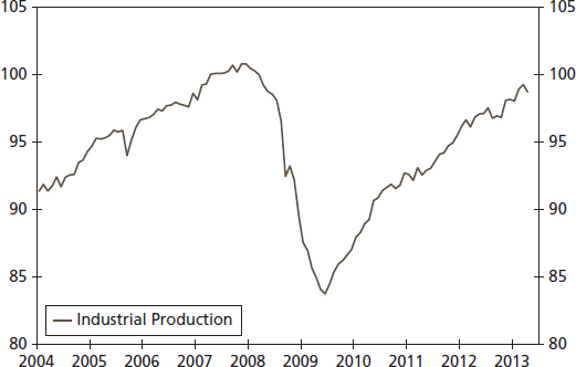
FIGURE 13.1 Industrial Production, Total Index (SIC) (Units 2007=100)

Source: Federal Reserve Board

For long-term forecasting, forecast errors and the potential need to rebuild the model depend on the nature of the shock (i.e., whether an economic shock creates a permanently shift in a series' trend or not). A shock can break the trend of a series. If the behavior of the series (e.g., upward or downward moving) remains the same as the pre- and post-break eras, then that break can be seen as a black swan. If, in contrast, a series depicts different behaviors for pre- and post-break periods, then the break can be labeled a group of black swans.⁵ The reason to divide the break into a black swan and a group of black swans is that the forecast errors would be different for the long-term forecasting models. An analyst would treat these shocks differently during the remodeling process.

Let's first explain a black swan and then a group of black swans.

In the case of a break in the trend, or a black swan, the movements in the trend would be similar for the pre-break and post-break eras. One example is the case of the U.S. Industrial Production (IP) data in Figure 13.1. During the January 2004–December 2007 period, the IP index had an upward linear trend. After December 2007, the trend experienced a break and the IP index started falling, eventually bottoming out in June 2009. Since July 2009, the IP index has returned to its linear upward trend that was consistent with the pre-December 2007 time period. This is an example of a black swan. The economic event, in this case the Great Recession, caused a momentary change in the growth pattern of the data. Eventually, however, the data returned to its long-run growth path.

FIGURE 13.2 A Group of Black Swans: A Shift in the Distribution

Source: Authors' calculations

Before we discuss the consequences of a black swan to long-term forecasting, let us explain the concept of a group of black swans. If the post-break era performs differently from the pre-break regime, we call it a group of black swans—that is, a shock caused a break in the trend of a variable that did not allow the variable to recover to its previous trend after the break. Put differently, the shock created a permanent shift in the distribution of a variable. The shift can be inward, outward, and so on; see Figure 13.2.

There are two examples of a group of black swans illustrated in Figures 13.3 and 13.4 where there is a shock to the economic system that drives both series into a very different model of behavior. In the first case, the shock shifted the trend of the series (unemployment rate) upward and it stayed there (see Figure 13.3). Clearly, the unemployment rate series have two different patterns: (a) before March 2008 (break date identified as the sudden shift in the average (mean) value of the time series, here the unemployment rate), the unemployment rate follows a decreasing trend and bottoms out at February 2008 and (b) after that break date, the unemployment rate rises quickly and peaked at October 2009. From October 2009 onward, the unemployment rate stayed at an elevated level compared to the historical standard. The mean and standard deviation of the pre-break date era (January 2004–February 2008) is 4.96 percent and 0.41 percent, respectively. For the March 2008–May 2013 period (after the break date), the mean is 8.40 percent and the standard deviation is 1.30 percent, both significantly higher than the values of the pre-break date era.

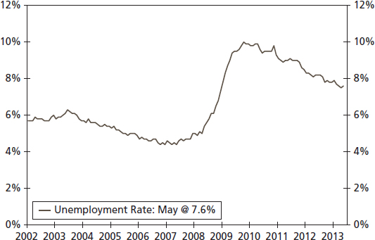
FIGURE 13.3 The Unemployment Rate

Source: U.S. Department of Labor

FIGURE 13.4 The S&P/Case-Shiller HPI

Source: Standard & Poor's and Case-Shiller

Figure 13.4, showing the S&P/Case-Shiller HPI, depicts the second example of a group of black swans. The index experienced an increasing trend until April 2006, which is the break date when home prices broke their upward trend and then prices started falling and the HPI bottomed out in April 2009. After this, the HPI did not return to the pattern of the pre-break (April 2006) era and displays a completely different pattern. In addition, the mean and standard deviation for the January 2002 to April 2006 (pre-break) era are 153.1 and 24.7, respectively. The mean of the post-break era is significantly smaller than that of the pre-break era, which is 132.6 (standard deviation is 4.34). A group of black swans can change the behavior of a series completely.

What are the issues and challenges posed by a single black swan and a group of black swans? In the case of a black swan, since a variable follows a consistent pattern with the pre-break era, the model used prior to the break date may still produce reliable forecasts. The reason is that a shock may break the trend, but the movements (upward or downward) would remain the same once a series bottoms out (or peaks). For instance, the IP peaked in December 2007 and then started falling before bottoming out in June 2009. After June 2009, the IP followed an upward trend consistent with the pre-December 2007 trend. Therefore, a model built for the pre-December 2007 era may be still appropriate to utilize, all else being equal. The issue, however, would be to know when a series is bottoming out. This implies that the forecaster must observe the target variable (IP index) and its potential predictors to judge the changes in the series.

The case of a group of black swans is more challenging because we do not know what pattern the series will follow in the post-break era. In the two examples provided in the previous section (unemployment rate and house prices), the post-break eras followed a different pattern from the pre-break periods. Therefore, the chances of uncertainty are much higher with a group of black swans than with a black swan. Another difference is that a forecaster is better off building a new model because the original model was built around relationships between variables that have likely broken down in the new economic environment. A new model, based on new relationships and new environments, will be needed.

For long-term forecasting, we suggest generating different scenarios instead of one forecast because the chances of a shock are higher. If the shock is a black swan, the old model may be utilized for forecasting. If the shock is a group of black swans, a new model must be built for future forecasting.

MODEL-BASED FORECASTING AND THE GREAT RECESSION/FINANCIAL CRISIS: WORST-CASE SCENARIO VERSUS PANIC

The Great Recession and financial crisis posed a great challenge to short-term and long-term model-based forecasting. Many economic and financial series experienced a structural break and became very volatile. The financial crisis raised many questions about the credibility of model-based forecasting.

We believe for three primary reasons that model-based forecasting remains a reliable tool in the decision-making process. First, model-based forecasting is an evolving and flexible process that allows for current-period information and future expectations to be incorporated in the model.

Second, in scenario-based forecasting, a forecaster generates different forecasts, including the worst-case scenario, to prepare for different future scenarios. However, there is always an even worse case within a worst-case scenario, more appropriately called a panic. There is a threshold between a worst-case scenario and a panic. Once the threshold is crossed, the worst-case scenario converts to a panic. Unfortunately, the threshold that converts a worst-case scenario into a panic is unknown. But analysts and decision makers can feel when a worst-case becomes a panic. Several panics occurred during the financial crisis. One was the failure of Lehman Brothers, which filed for bankruptcy on September 15, 2008, igniting the global financial meltdown. Lehman's bankruptcy triggered a series of global events that included bank failures across the world. Lehman's collapse turned the worst-case scenario into a panic. Typically, financial institutions have reserves to deal with uncertain situations (worst-case scenarios); when people lose confidence in these institutions, it is hard for those banks to survive as a run on them ensues. This is a panic. In the case of a panic, financial institutions are unable to do anything except for file for bankruptcy. Therefore, in our view, the panic during the financial crisis was a major cause of the failure of forecasts.

Unfortunately, in the case of a panic, a forecaster is unable to do much in terms of predictions. But there is much to be learned after a panic.

Finally, economies tend to reach a new equilibrium where new economic relationships tend to be established. Only rarely do economic systems become explosive and collapse leading to a complete break in economic organizations—Weimar Germany being a notable example. Since a new set of economic relationships tend to be established, the employment of model-based-forecasting becomes effective once more.

SUMMARY

Model-based forecasting, whether short term or long term, consists of three phases: modeling, assessing, and remodeling. It is critical that the forecaster continuously monitors and analyzes the performance of the model and, if inaccuracy persists, rebuilds it.

In certain cases, more common in short-term forecasting, due to temporary events, a forecaster would need to incorporate add factors into the model to reduce forecast error. In some cases, remodeling will not be necessary. In long-term forecasting, we suggest producing multiple scenario-based forecasts instead of a single forecast. In addition, the nature of a break (think black swan or a group of black swans) determines whether the forecaster will need to construct a new model.