CHAPTER 14

Putting the Analysis to Work in the Twenty-First-Century Economy

During the current business recovery, the economic performance of the United States has been very different from what many analysts had expected. Decision makers in both private and public sectors faced a set of mixed economic and financial indicators that offered a confused picture of the state of the economic recovery, the pace of that recovery, and the character of the structural challenges facing the economy.

At the start of America's journey to recovery, three major trends characterized the confusion. First, gross domestic product (GDP) growth had been unusually low and uneven relative to economic recoveries since World War II. During the recovery, the economy accelerated after an initial stimulus from the Federal Reserve (the Fed) and the federal government but then lost momentum as the stimulus generated no follow-on acceleration in growth. Decision makers had the difficult challenge of identifying what was the true trend in the economy and what was the cycle around that trend. Had trend economic growth fundamentally downshifted in the United States?

Second, job growth had become the number one political issue for both parties. But job growth appeared soft and out of line with GDP growth as the business cycle progressed. Further, weak job growth intimated a sharp structural break in both private and public sector decision makers' preconceived understanding of the relationship between employment and population growth, where employment levels rose alongside population growth. Had there been a structural break between employment and population growth and/or between employment and output growth? Why have exceptionally low mortgage interest rates not spurred a pickup in housing, as in prior recoveries? Had this relationship experienced a structural break as well?

Third, corporate profits, business equipment spending, and industrial production improved in this cycle in a way reminiscent of prior recoveries despite the overall perception that the economic recovery had been subpar. How can we identify economic series that appear to behave in typical cyclical fashion compared to those that do not?

In this final chapter, we look at the benchmark economic series that frame good decision making: output, employment, profits, interest rates, and the dollar exchange rate.

To address these issues effectively, let's recall our work returns to an earlier tradition of applied research. In contrast, our approach in this text differs from the theoretical econometrics text, which is almost all technique with little to no real-world application, or an economics text with primarily economic theory approach with no applied techniques and only hypotheses about economic behavior in the real world.

Due to the Great Recession (2007–2009) and the accompanying financial crisis, the need for effective economic analysis, especially the identification of time series and then accurate forecasting of economic and financial variables, has significantly increased. Our approach provides a comprehensive yet practical process to quantify and accurately forecast key economic and financial variables.

Different economic and financial variables—economic growth, final sales, employment, inflation, interest rates, corporate profits, financial ratios, and the exchange value of the dollar—exhibit differential behavior over the business cycle and over time.

A strategic vision with a context for where the economy is headed is thus needed. This vision requires the effective application of time series techniques to address both private and public sector decisions. Economic analysis is an essential element in effective due diligence, and our focus emphasizes the five key economic fundamentals: growth, inflation, interest rates, profits, and the dollar.

BENCHMARKING ECONOMIC GROWTH

Throughout this chapter, we discuss the various elements of bias in decision making. With respect to projecting the growth of the economy, the presence of an anchoring bias must be recognized. This bias makes its appearance as an analyst anchors expectations of the future based on an anticipation that it will look a lot like the past. Expressed differently, does the path of the mean of a series revert back to a past value after a shock?¹

Our view is that the U.S. economy's growth from the 1950s through the mid-1970s reflected a closed economy with a store of savings from the World War II era and a history of low inflation and interest rates. However, the context of the economy differs markedly today. Since the mid-1970s, the global price of energy has risen dramatically. Changes in Canadian and Japanese trade policy have introduced competition into many sectors. This global competition aspect has been magnified with the North American Free Trade Agreement, and the rise of China as a major economic power and its entrance into the World Trade Organization has also increased competition. The evolution of the economy represents a constant challenge to the temptation to anchor analysis to the past. Here we begin a test for mean reversion in the post-inflation era beginning in 1982.

Benchmarks: Economic Growth and the Labor Market

To provide better guidance for decision makers, we focus on two broad areas of the U.S. economy: economic growth (output) and the labor market. The Great Recession produced the largest losses in terms of output (as measured by GDP) and jobs (nonfarm payrolls) in the post–World War II era. After experiencing such deep and severe losses, can the economy ever get back to the “normal” level? Will we see mean reversion? To answer these questions, we test the behavior of U.S. GDP and industrial production to proxy output in the economy and two indicators of the labor market: the unemployment rate and nonfarm payrolls.

Testing, Not Assuming, Economic Values for Good Decision Making

Fortunately for decision makers, econometric techniques can frame the behavior of strategic variables that define our economic baseline for strategy. Here we wish to determine whether a series is mean reverting. In Chapter 4 we introduced the concept of unit root testing and our preferred test, the augmented Dickey-Fuller (ADF) test, as the process to quantify whether a series is mean reverting. Recall that the null hypothesis of the ADF test is that the underlying series is not mean reverting (nonstationary) and the alternative hypothesis is that the data series is mean reverting (stationary). If a series is nonstationary, then the behavior or change from one period to another is random and the future values are unpredictable.

FIGURE 14.1 Real GDP Growth: Compound Annual Growth Rate

Source: U.S. Department of Commerce and authors' calculations

The goal of a forecaster is to predict the movement of data over time. To evaluate the movement of a time series, a decision maker can employ ordinary least squares (OLS) regression analysis, which will provide the estimated mean value of the time series. However, since stationarity of the data, or constant variance, is a critical assumption of OLS regression, we utilize the ADF unit root test to evaluate whether we can take the mean as given or if the results are spurious. If the ADF test proves the data to be nonstationary, then we have violated an underlying assumption of OLS regression analysis and cannot draw any conclusions from the results. However, if the ADF test proves the data to be stationary, the next step is to define the stationary behavior of the data. Three possibilities exist regarding stationary behavior. A data series can be: zero mean, which identifies the mean of the data series as zero; single mean, which defines the data series as having a constant mean that is not zero; and trend growth, meaning that the data series does not have a constant mean over the time period but follows a consistent time trend with finite error terms. Examining the time series in chart form is often very helpful in determining the form of stationarity of that data series.

Our Benchmark for Real GDP Growth: 2.75 Percent

Over the sample period, Q1-1982 to Q4-2012, the average annualized growth rate of real GDP in the United States was 2.75 percent, as illustrated in Figure 14.1 and confirmed with the OLS analysis in Table 14.1. Is this a reasonable benchmark to guide our expectations? The results in Table 14.1 show no evidence of a shift or long-term deviation from the long-run average rate of GDP growth. Therefore, the GDP data series appears stationary and exhibits mean reversion back to its 2.75 percent value.

TABLE 14.1 GDP ADF Results Exhibit Stationarity

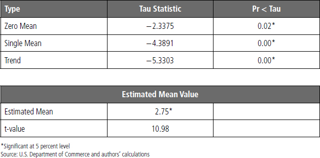
In the ADF unit root test illustrated in the top portion of Table 14.1, we can reject the null hypothesis of mean diversion or nonstationary growth of GDP at the 5 percent significance level.² While the table demonstrates the possibility of zero mean, single mean, and trend growth, we identify the series as single mean using the value of the mean from the OLS analysis. The OLS analysis finds that a mean of 2.75 percent is significant, and the chart also confirms our suspicions of a mean-reverting data series around 2.75 percent.

We can thus conclude that GDP growth is mean reverting. For decision makers, the benchmark for strategic thinking is that growth will more likely be 2.75 percent over time; therefore, divergent views from this growth rate are less than an even bet. This is especially true for outlooks beyond the next two years that really reflect the longer-term trend of growth. In this case, the trend is more likely to fall around 2.75 percent rather than values such as 4 percent plus or a drop to zero growth. Finally, the evidence, so far, does not imply a fundamental downshift in economic growth in recent years, even though the average growth rate has been below 2.75 percent for several years. There is just not enough evidence to advocate a fundamental, statistically significant, shift in the growth rate of GDP.

FIGURE 14.2 Industrial Production: Compound Annual Growth Rate

Source: Federal Reserve Board and authors' calculations

INDUSTRIAL PRODUCTION: ANOTHER CASE OF STATIONARY BEHAVIOR

In a similar way, the OLS regression analysis estimates an average quarterly annualized growth rate of 2.29 percent for industrial production over the sample period. The unit root test demonstrates that industrial production data is stationary; therefore, we can validate the long-run average growth of industrial production to remain around 2.29 percent. As can be seen in Figure 14.2, industrial production growth demonstrates a cyclical pattern—falling during recession and bouncing back during the early phases of recovery as we reviewed in Chapter 1. However, these anticipated deviations from the long-run mean are temporary in nature. Therefore, a decision maker can anticipate industrial production growth around its long-term trend despite its cyclical pattern. Table 14.2 illustrates the results of our test for stationarity, which indicates that the industrial production growth series is stationary over time despite the constant ups and downs over various business cycles.

Decisions based on any movement away from the mean of stationary series are subject to a confirmation bias—the tendency of an observer to view new information in a way that confirms the observer's prior beliefs. Earlier in this economic recovery, we witnessed three examples of the confirmation bias in action. First, as illustrated in Figure 14.3, real GDP rose sharply with the initial fiscal stimulus program in 2009. However, this pace of growth was not sustained as growth quickly moderated to a 2 percent pace, where it has remained throughout this economic expansion.

TABLE 14.2 ADF Results Indicate Stationarity for Industrial Production(2)

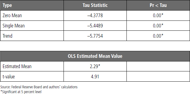
FIGURE 14.3 Real GDP: Compound Annual Growth Rate

Source: U.S. Department of Commerce

In a similar way, existing homes sales jumped in 2009 in response to the enactment of the first-time home buyer credit.³ As evidenced in the Figure 14.4, the jump in sales was quickly eroded and did not sustain a recovery in existing home sales. The Cash for Clunkers program gave rise to a sharp jump in light vehicle sales but then was followed by a sharp drop-off and very little sustained improvement in sales the next two years (see Figure 14.5).⁴ The confirmation bias comes into play when the early successes of these or any change in trends are extrapolated by proponents into permanent changes in the pace of economic activity. In economics, the general principle demonstrated here is that temporary programs do not alter long-run behavior of households or businesses.

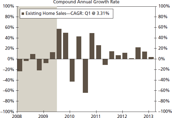
FIGURE 14.4 Existing Home Sales

Source: U.S. Department of Commerce

EMPLOYMENT: JOBS IN THE TWENTY-FIRST CENTURY

Growth in employment stands as a primary input for any accurate estimate of the state of the American consumer. Retail and auto sales for the private sector, sales tax revenues/auto registrations for state and local government, and federal payroll and income taxes are three estimates that start with job gains. Meanwhile, policy goals for the Federal Reserve, the president, and Congress are defined by their ability to reach certain levels of unemployment and monthly job gains. Finally, the impact of many policy actions, such as regulations, minimum wage changes, and eligibility for certain programs such as disability payments, are benchmarked by their impact on the job market. For policy makers in the current recovery, the behavior of the unemployment rate has become the standard to judge the effectiveness of economic policy. We begin here.

FIGURE 14.5 Light Vehicle Sales

Source: U.S. Department of Commerce

Unemployment Rate Measured by U-3: A Surprising Result

The unemployment rate, measured by the U-3 definition that is commonly reported in the media and serves as a benchmark for stress testing advocated by the Federal Reserve, displays stationarity (see Figure 14.6).⁵ These results may be surprising to some commentators and decision makers, especially given the persistently high, and seemingly outsized, unemployment rates since the latest recession. The results in Table 14.3 indicate that the official unemployment rate is mean reverting around a long-term average rate of 6.37 percent. The long-run average is surprisingly close to the Federal Reserve's guidepost of 6.5 percent for raising the federal funds rate.

Unfortunately, an unemployment rate of 6.375 is higher than what is perceived as full employment by those with an anchoring bias looking at the past. Yet our statistical evidence indicates that the unemployment series does not exhibit any drift in the values over time since 1982 and implies that perceptions that the long-term level of unemployment has shifted upward since the Great Recession are misplaced. So far no statistical evidence exists of a fundamental shift in this series in the post-recession period.

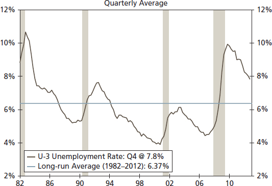
FIGURE 14.6 Unemployment Rate: U-3

Source: U.S. Department of Labor and authors' calculations

TABLE 14.3 Stationarity For the U-3 Measure of Unemployment: The ADF Results

Employment Growth: Surprisingly Stationary Despite Impressions

In addition, we find that the growth in payrolls (see Figure 14.7) is surprisingly stationary. Public impressions today fall prey to the recency bias that assumes that the most recent experience is a signal of the future that is distinct from the past.⁶ Yet the evidence shows that the annualized quarterly growth rate of nonfarm employment is actually a stationary series that is mean reverting. The average growth rate is estimated at 1.28 percent over the Q1-1982 to Q4-2012 period. In Q4-2012, payrolls were growing at a 1.64 annualized rate, above the long-term trend.

FIGURE 14.7 Nonfarm Payrolls

Source: U.S. Department of Labor, and authors' calculations

In Table 14.4, we show the statistical test results indicating stationarity of the growth in payroll employment over the sample period. This would appear surprising to those analysts who focus on the variation over the cycle. Here, however, we are more interested in the trend over time and that trend growth rate appears to be stationary over the sample period.

Patterns of employment open up the door to biases in decision making that may lead us astray. In Figure 14.8, the monthly gains in nonfarm employment are illustrated for the current recovery. While our earlier statistical analysis would indicate stationarity in the growth of employment, some took the spike in employment by hiring Census workers in 2010 as a signal of a robust job market. Why? Unfortunately, the job gains coincided with some analysts' projections that the fiscal stimulus would lead to a rapid gain in economic growth in 2010. For decision makers, this is an excellent example of the confirmation bias—the interpretation of data/observations as a confirmation of an anticipated outcome. Some analysts anticipated job gains, they saw some job gains, and therefore they judged the economy to be taking on the path of rapid growth. Yet the pattern of employment after the spring of 2010 did not show any evidence of this prediction.

TABLE 14.4 Employment Growth as a Stationary Series: The ADF Results

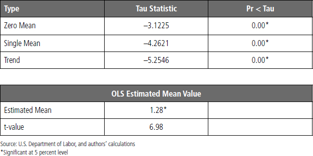
FIGURE 14.8 Nonfarm Employment Change

Source: U.S. Department of Labor

The change in character of the U.S. labor market is also evident by the rise in the proportion of the labor force that is composed of part-time workers and the rise in underemployment where many workers are in jobs below their level of education and skills. Further evidence of the structural change in the labor market is revealed in the following discussion on the Beveridge curve.

FIGURE 14.9 Beveridge Curve in Employment Recoveries

Source: U.S. Department of Labor

The Beveridge Curve: Yet to Shift Inward

While some analysts have argued that the structural shift in labor markets, as evidenced by the Beveridge curve, is a temporary cyclical phenomenon, after four years of economic expansion, this shift seems like a more fundamental change.⁷ Even as the headline U-3 unemployment rate has improved in the typical, albeit slow, cyclical fashion, other labor market indicators suggest that today's labor market environment has changed. Job vacancies have become more plentiful as the economy has recovered. However, as shown in Figure 14.9, the unemployment rate remains high relative to the rate of job openings in previous cycles and intimates more frictions in matching the unemployed with available jobs.

It has been argued that the outward swing in the Beveridge curve is typical during the early stages of a labor market recovery. While some skills mismatch is normal as the economy undergoes significant periods of restructuring following a recession, more than four years into the recovery, the Beveridge curve remains above its path during the last economic expansion. The Great Recession a challenge to structural frictions beyond the typical pattern. The share of unemployed workers out of a job for more than 27 weeks remains historically high. The longer these workers are out of a job, the higher the risk that the slow cyclical recovery results in a longer-lasting structural mismatch as these workers' skills become increasingly out of date.

FIGURE 14.10 Employment–Population Ratio

Source: U.S. Department of Labor

Structural Change in the U.S. Labor Market: Two Illustrations

Two indications of structural change in the labor market not captured by apparent stationarity of the U-3 unemployment rate are the sharp downdraft in the employment–population ratio (see Figure 14.10) and the decline in the labor force participation rate (see Figure 14.11).

According to the employment-population ratio, there are far fewer workers as a share of the working-age population than in the past. This creates two problems. First, to achieve any given pace of economic output, productivity must improve significantly for the fewer current workers. Second, when inverted, this employment-population ratio hints that a far smaller share of the population is supporting the rest of the population through government spending, especially entitlement programs, than in the past.

Structural change in the labor market not captured by the U-3 unemployment measure is also indicated by the drop in labor force participation (see Figure 14.11). In recent years, a decline in labor force participation for both male and female workers reinforces the view that the future pace of GDP growth may downshift from current perceptions. This downshift in future economic growth represents a challenge to decision makers. Many analysts will ignore the changes in the labor market and its implications. Anchored in the past, they have a biased, out-date-view of the labor market, which leads to an overestimate of potential future economic growth as well as the potential of that growth to solve the structural unemployment problems of today.

FIGURE 14.11 Labor Force Participation Rate

Source: U.S. Department of Labor

Decision makers are also subject to the availability bias in their view of the labor market by judging the state of the economy on the most visible, available statistic—the U-3 unemployment rate. They fail to recognize the problems of underemployment, as represented by the U-6 statistics (which are less visible to many observers but also more accurate representations of the true nature of the economy). These problems include the increasing substitution of part-time for full-time employment and the mobility problems of many workers due to depressed home prices or skills mismatch.

INFLATION

Inflation measures are a major input to the cost-of-living adjustments to programs such as Social Security and in the setting of wage and benefits compensation baselines in the private sector. Inflation assumptions also impact estimates of valuation for financial assets. For example, despite current commentary that inflation is low, inflation still is in excess of returns to savers in money market funds and short-maturity U.S. Treasury bills and notes. It thus influences the investment behavior of investors and the flow of funds in the U.S. economy.

In the past, the pattern of inflation has influenced decision makers, especially investors, and has given rise to the recency bias that we need to recognize, given that inflation cycles evolve over time and that a focus on the recent behavior of inflation leaves us open to missing the next move of inflation in the future. For example, in the early 1980s, inflation expectations were based on the high inflation rates of the 1970s not changes in monetary policy under Fed chairman Paul Volcker and the conservative philosophy of President Ronald Reagan and his drive to cut taxes. Without this perspective, decision makers could not recognize that the future pattern of inflation would be very different and lower going forward. Those influenced by the recency bias bases future expectations on the most recent past information without allowing for changes in the economy.

FIGURE 14.12 TIPS Inflation Compensation

Source: Federal Reserve Board and University of Michigan

Inflation and Inflation Expectations

Investors should examine the argument that inflation expectations are well anchored more closely. We believe that investors should follow the observation of David Romer: Monetary policy has an inherent inflationary bias.⁸

One measure of inflation expectations is the five-year implied inflation expectations from the Treasury Inflation-Protected Securities (TIPS) yield, illustrated in Figure 14.12. This figure indicates that, since 2010, there has been a steady but very modest rise in inflation expectations. As implied earlier, inflation expectations are rising but not at the pace that would likely prompt any change in monetary policy soon. Whether these patterns indicate that inflation expectations are well anchored is another issue. More important for decision makers, the recent pattern of rising inflation expectations, although modest, intimates that nominal yields may not cover the actual inflation experience over time, a fact that must be brought into the investment calculus.

FIGURE 14.13 Inflation and the Real Yield

Source: Federal Reserve Board and University of Michigan

In Figure 14.13, inflation expectations, as measured from a University of Michigan survey, appear well anchored—unfortunately too well anchored. The series appears to stay remarkably close to 3 percent inflation, leaving little reason for policy tightening or easing over the past 16 years. Certainly there is no case for Fed actions to fight deflation fears in 2002 to 2004 or in 2007 to 2008. Yet the Fed took aggressive action through expanding its balance sheet. If this series is perhaps a benchmark for inflation expectations, then it should work on both the upside and the downside. Analysts who are complacent today may face a rude shock when inflation makes an unscripted return.

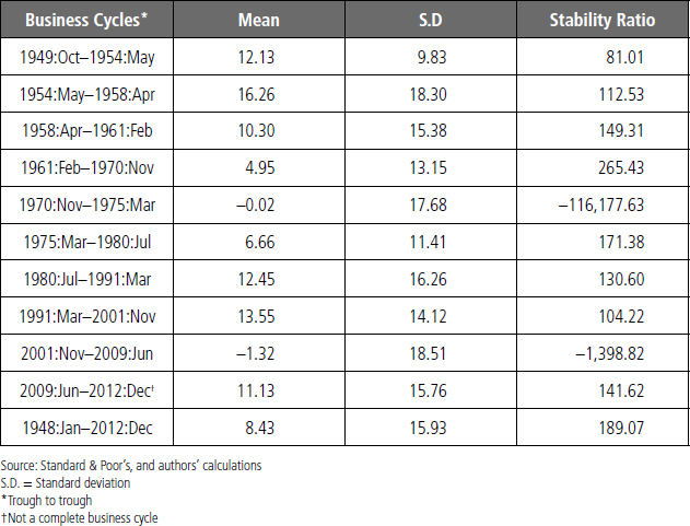
One cautionary note for decision makers: The perceived volatility in inflation is actually higher when the average inflation rate is lower, which sets up a position that the risk of inflation volatility is actually greater. This result will surprise many analysts. As shown in Table 14.5, the stability ratio actually has been higher in recent business cycles. Counterintuitive but true nonetheless.

Inflation: A (Small) Bias to the Upside

Current modest inflation, as measured by the consumer price index and illustrated in Figure 14.14, provides time for credit markets to continue to improve and also allows the Fed to continue current policy. A few market signals hint that inflation pressures are rising, although they are still not at a pace that would prompt the Federal Open Market Committee which sets monetary policy at the Federal Reserve System to alter its current policy.

TABLE 14.5 Business Cycles and Consumer Inflation

FIGURE 14.14 U.S. Consumer Price Index

Source: U.S. Department of Labor

Ten-year inflation expectations, Figure 14.15, have trended upward since 2010 and currently have returned to the levels that existed prior to the recession of 2007 to 2009. Similar to the five-year measure of inflation expectations, the current level of inflation expectations is not high enough to move the Federal Open Market Committee to alter its current policy.

Finally, gold prices have risen steadily since the recovery began in 2009, yet have leveled off in 2012 (see Figure 14.16). Gold prices, like many other prices, respond to several factors beyond overall inflation expectations. But many analysts utilize gold prices as an inflation proxy, and the message from gold prices now is that inflation n expectations do not appear to be accelerating. Moreover, gold is a globally traded commodity and is not well correlated to the pace of domestic inflation in the United States, as illustrated in Figure 14.17.

FIGURE 14.15 10-Year Implied Inflation Expectations

Source: Federal Reserve Board

FIGURE 14.16 Gold Price

Source: Bloomberg LP

Finally, Figure 14.18 demonstrates the rapid decline in velocity, or the turnover of money in the economy, as measured by the ratio of nominal GDP to the M2 measure of the money supply where M2 includes checking, savings and money market funds for example. This decline in velocity illustrates the break down in the link between money and inflation. While this relationship appeared very strong even over short periods in the 1960s and 1970s, it began to crumble in the 1980s. This fact again shows that some analysts continue to succumb to their anchoring bias and base their projections of inflation on their experience from decades ago. The global economy has evolved in such a way that the U.S. currency is employed globally, reducing the domestic link of money to inflation. Analysts would be better served if they developed a model for inflation going forward, a rational expectations approach, that reflects the changing character of the application of money in the global economy and the myriad of influences on inflation in the short and long run.⁹

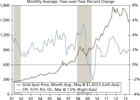
FIGURE 14.17 Gold Spot Price and Price Inflation

Source: Bloomberg LP and U.S. Department of Labor

FIGURE 14.18 M2 Money Supply Velocity

Source: Federal Reserve Board and U.S. Department of Commerce

INTEREST RATES

Interest rates and changes in those rates, both anticipated and unanticipated, are two of the driving forces of economic activity. Our focus on the role of interest rates as the price of credit reflects the realization that interest rates are a major factor influencing the pace of home purchases and refinances. During the last decade, fluctuations in the level of interest rates were a major force supporting both the boom and the bust in housing. For the business sector, interest rates represent one cost of credit or capital and a hurdle that an investment must overcome if that investment is to be pursued.

For investors, interest rates indicate the rate of return on savings accounts, money market accounts, and fixed income investments such as public and private bonds. For state and local governments, interest rates are the cost of borrowing, which is often benchmarked off the yield on Treasury interest rates. We turn to those rates shortly.

Interest rate expectations are subject to a set of biases for decision makers that can be, and have been, very expensive in terms of economic performance. During the 1970s, inflation rapidly outpaced interest rates, and real interest rates were negative. At the time, analysts rationalized this deviance (the normalization of deviance) in traditional behavior (nominal interest rates typically exceed inflation) to their own cost as rapid inflation and interest rate increases later in the decade led to large capital losses for investors. Early in the 1980s, many analysts complained that the level of interest rates was too low and that interest rates, along with inflation, would rise quickly as the economy picked up steam and the Fed loosened up on the money supply. This return to the past represented the anchoring bias.

Today, with inflation again outpacing the level of short-term interest rates, decision makers are again faced with the challenge that the current environment is not sustainable over time. In addition, the pace of home price increases is once again exceeding mortgage rates, which is reminiscent of the period from 2004 to 2007. Is another housing bubble looming? These issues require an assessment of the balance between real and nominal interest rates to which we now turn.

FIGURE 14.19 Inflation and the Real Yield

Source: Federal Reserve Board and University of Michigan

Inflation and Real Yields: A Signal of Financial Imbalances

From our viewpoint, one sign of financial imbalances in the economy is the extent to which inflation expectations are not reflected in current five-year Treasury yields (see Figure 14.19). In the early years of an economic recovery, Treasury yields often decline in line with easing monetary policy, as evidenced in 2002 to 2004. However, the current period indicates that yields are far below inflation expectations and have been there for some time. This shows that the extent of Fed buying of Treasury debt, along with purchases of U.S. Treasury debt by the Japanese and Chinese central banks, has distorted pricing in the Treasury market.

IMBALANCES BETWEEN BOND YIELDS AND EQUITY EARNINGS

Another signal of the unusual circumstances in today's capital markets is the inversion in the ratio between Baa corporate bond yields and Standard & Poor's (S&P) earnings, as illustrated in Figure 14.20. Bond yields appear low relative to equity earnings, even though general equities have historically yielded more (1990–2007) and are considered riskier investments.

Credit default swap (CDS) premiums provide the analyst a measure of the risk assessment in the marketplace for any financial instrument. A CDS is a financial agreement that the seller of the CDS will compensate the buyer in the event of a loan default or other credit event (e.g., a downgrade). The buyer of the CDS makes a series of payments (the CDS “fee” or “spread”) to the seller and, in exchange, receives a payoff if the loan defaults.

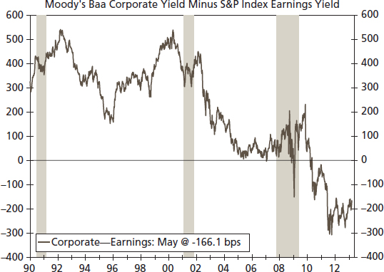
FIGURE 14.20 Baa Corporate Yield over S&P Index Earnings

Source: Moody's Analytics, S&P

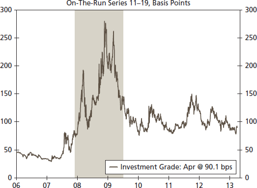
FIGURE 14.21 Investment-Grade CDS Index

Source: Mark-It Partners and Bloomberg LP

In Figure 14.21, these premiums spiked during the recession period to reflect the rapid rise in the risk that an issuer of investment grade bonds might default or would be downgraded. In addition, spreads in the post-recession period remain wider relative to the spreads prior to the latest recession. This suggests that market participants have adjusted their risk assessments to be a bit more risk averse than before the recession and reflects an adjustment in risk perceptions that would nullify the anchoring bias that might have led to a return to prior narrow spreads.

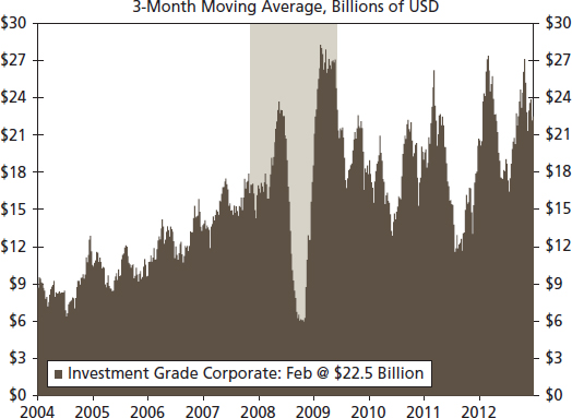
FIGURE 14.22 Investment-Grade Corporate Issuance

Source: IFR Markets

Healthy Bond Issuance Consistent with Functioning Credit Market Expansion

Bond issuance in 2012 was a strong signal that credit markets were again functioning normally. As illustrated in Figure 14.22, investment-grade bond issuance has been at a consistent and solid pace for several years now. In addition, high yield issuance (see Figure 14.23) has accelerated in recent years as the recovery/expansion matures. These developments support our view that credit markets are functioning normally as far as the corporate bond market is concerned.

Unfortunately, there are now new worries for bondholders.¹⁰ Low interest rates and more optimistic views of the economy, compounded by an accommodating bond market as illustrated by the strength of issuance, has given some investors the opportunity to pursue leveraged buy-outs. These buy-outs, financed by debt issuance, could possibly lead to downgrades of corporate debt and investor losses. At present, the risk of leveraging activity has increased. Decision makers need to consider whether the current low-interest-rate policy has stayed too long and thereby is encouraging a more aggressive risk-taking appetite than perhaps the Fed anticipated.¹¹

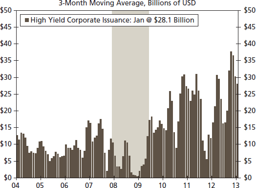
FIGURE 14.23 High-Yield Corporate Issuance

Source: IFR Markets

Finally, current Aaa and Baa corporate bond spreads (see Figure 14.24) have traveled in a range slightly higher than during the boom period of 2005–2006, indicating that a risk premium in the market today provides a better risk/return balance than during the boom period. It is reassuring that the market is pricing risk in a better way than it did in the past decade.

Two-Year Treasury Yield: Benchmark for the Short End of Yield Curve

Over the sample period, Q1-1982 to Q4-2012, the two-year Treasury yield, expressed commonly in level form, was nonstationary. That is, the two-year Treasury yield actually declined over the sample period, as illustrated in Figure 14.25 and this decline was statistically significant. The two-year Treasury yield, reflects the expected path of interest rates over the next eight quarters since, for example, an investor could buy a one-year Treasury bill and then reinvest those proceeds with the result that her return on that strategy would equal the return on the two-year note today. This two-year yield then indicates the expected path of interest rates and that is critical for decision makers to judge their expected financing costs over this two-year period.

FIGURE 14.24 Aaa and Baa Corporate Bond Spreads

Source: IHS Global Insight

FIGURE 14.252-Year Treasury Yield

Source: Federal Reserve Board and authors' calculations

TABLE 14.6 Evidence of Nonstationarity of the Two-Year Yield: ADF Results

In the augmented Dickey-Fuller unit root tests illustrated in Table 14.6, the probability of a unit root at a 5 percent level of significance implies that we cannot reject the null hypothesis of the nonstationary character of the level value of the two-year Treasury yield that appears in so many economic surveys. Therefore, the two-year Treasury rate is not mean reverting and, as can be seen in Figure 14.25, has followed a downward time trend. Formal trend testing reveals that the two-year Treasury yield has a linear, downward trend over our sample time period.

For decision makers, the benchmark for strategic thinking for the two-year Treasury yield is that it is not mean reverting. Therefore, a thoughtful economic estimate would have to alter the two-year yield level in some way to generate a stationary series.

Adjusting the Two-Year Treasury Yield to Achieve Stationarity

Once we have identified that a series, the two-year Treasury yield in our case, is nonstationary at level form, then we need to determine the type/source of nonstationarity. Recall that that there are two major types of nonstationary behavior: difference stationary (DS) and trend stationary (TS). It is important to identify the character of a time series as either DS or TS because both sources of nonstationarity have different implications for the future path of the variable. If a series follows the DS pattern, then the effect of any shock will be permanent. To convert the series into a stationary process, an analyst would have to generate the first difference of the series. A common source of nonstationarity is TS behavior, which implies that the series has a deterministic trend (upward or downward) over time. To convert a TS series into a stationary form, we have to de-trend the series, meaning regress the variable of interest on a time dummy variable.¹²

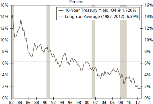
FIGURE 14.26 10-Year Treasury Yield

Source: Federal Reserve Board and authors' calculations

The two-year Treasury series appears to exhibit TS behavior, implying that it does not have a constant mean; the mean changes over time and a benchmark average rate for the two-year Treasury yield should not be applied to future forecasts. We propose that the two-year Treasury yield contains a TS behavior for two reasons: (1) The graph of the series (see Figure 14.25) shows a clear deterministic downward trend; and (2) we employed regression analysis to determine the type of trend (i.e., to determine whether the trend is linear [constant growth rate over time], nonlinear [nonconstant growth rate], or log-linear [the log of the series has a constant growth rate]). The regression results indicate that the two-year Treasury yield contains a linear downward time trend.

10-Year Treasury Yields: Not Mean Reverting

In a similar way, when expressed in level form, the 10-year Treasury yield (see Figure 14.26) is a nonstationary series with trend behavior. As illustrated in Table 14.7, the probability calculation, Pr < Tau, is significantly greater than the 5 percent significance level for both the zero mean and the single mean, such that we cannot reject the hypothesis of a unit root or nonstationary behavior of the 10-year Treasury yield. But the Pr < Tau is less than 0.05 in the case of “trend,” indicating the 10-year Treasury rate contains TS behavior.

TABLE 14.7 Ten-Year Treasury: The ADF Results

Once again, we can achieve stationarity for the 10-year Treasury yield series by de-trending the series. Regression results imply that a nonlinear (U-shaped) trend better fits the series. That is, a de-trended 10-year Treasury rate is mean reverting and thereby can be utilized in the econometric analysis and forecasting.

A NOTE OF CAUTION ON PATTERNS OF INTEREST RATES

While the pattern for interest rates on 2- and 10-year Treasury securities has been a gradual decline since 1982, there is also a question of the longer-term cycles in interest rates in history. For example, interest rates rose steadily from 1900 to 1920 and again from 1946 to 1981. In contrast, rates fell steadily between 1920 and 1946 and, of course, in the recent period. As a result, analysts must put any trend in rates in the context of the longer-term movements in the economy, inflation, and the overall credit markets.

In his seminal paper on business cycle modeling, Nobel Prize–winning economist Robert E. Lucas reinforced this message by finding that the welfare gain from stabilization policy is small.¹³ While the benefits from stabilization may be greater than what Lucas cites (see Clark, Laxton, and Rose, 1996), there does not appear to be a clear case for a stabilization policy that seeks growth above a trend pace of 2.75 percent and also does not account for the distortions created in the credit markets at the same time when those stabilization efforts are undertaken.¹⁴

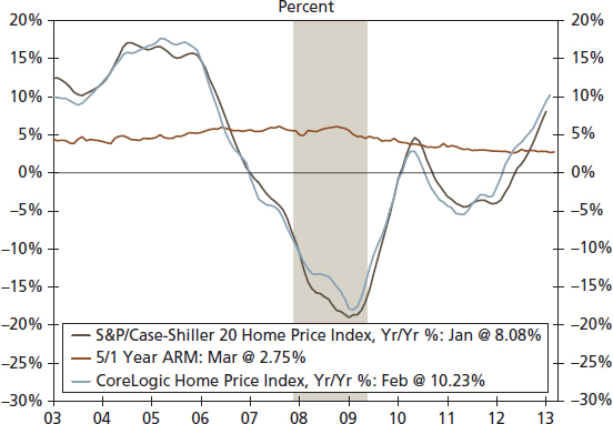
FIGURE 14.27 Home Price Growth versus Mortgage Rates

Source: Standard & Poor's, Bloomberg LP, and CoreLogic

For investors and decision makers, we would advocate a high degree of skepticism regarding the claim that there is no evidence that U.S. central bank purchases have impaired the functioning of financial markets (and the real economy as well). In fact, we see distortions developing in the housing market today similar to those that gave rise to the housing boom of 2004 to 2007. As evidenced in Figure 14.27, the current pace of home price inflation exceeds the going rate on home mortgages—as was the case during the period from 2004 to 2006. In effect, home price inflation is increasing faster than the rise in the burden of home finance, which is exactly the problem that gave rise to prior housing excesses. It is possible, therefore, that housing decisions are in fact being distorted.

Decision makers need to give greater thought to tempering purchases of mortgage-backed securities as the level of housing starts are not part of the Fed's mandate. The housing market reflects the experience of two-decision making biases that analysts must recognize:

1. The traditional model of monetary policy easing led to lower interest rates, and a housing rebound did not occur with anything like the response many analysts expected. Instead, the responsiveness of housing was very weak, reflecting the anchoring bias of analysts who rely on models based on past behavior rather than recognizing changes in the economy during the recent 2009–2012 period and therefore reflecting the context of the economy (lower consumer confidence) and credit markets (restrictions on bank capital and new bank lending regulations) around any easing policy at that time.
2. The home price decline created a sunk cost bias among homeowners to sell their home at a loss.

FIGURE 14.28 Commercial and Industrial Loans by Bank Type

Source: Federal Reserve Board

Both biases reflect thinking that was not in vogue prior to the recession, and therefore are warnings to analysts to recognize the constant evolution of the economy over time.

Whereas the role of a central bank is to provide liquidity when needed, and we have ample liquidity in markets today, specifically targeting housing and how Fed supplied credit market liquidity is employed will create pricing distortions for investors and decision makers alike.

BUSINESS CREDIT: PATTERNS REMINISCENT OF CYCLICAL RECOVERY

Finally, the gains in commercial and industrial loans for all three categories of banks (see Figure 14.28) indicate that credit is being made available. For some analysts, this fact reduces the case that further aggressive policy easing is needed. Here, in contrast to housing, business lending appears to be taking on the pattern of a cyclical recovery and does not provide evidence of a structural break in credit availability.

PROFITS

Profits are rewards for economic success and incentives for innovation and change in the business sector. Profits also provide the source of capital for investments that will increase productivity and the standard of living for any society over time. However, profits are very cyclical. Interpreting short-term trends in profits can lead to extrapolations of recent profit gains that would be inconsistent with the cyclical character of profit growth. For example, above-average profit growth in the early phase of the economic recovery tends to encourage analysts to extrapolate into the future. This is the familiar pattern of the bias of the normalization of deviance, where deviations from trend, on both the upside and the downside, are treated as new trends. In a bull market for equities, prices and earnings can only go up. In a recession, prices and profits will never recover. Such are the sentiments of fear and greed in the market. As the next analysis illustrates, the share of GDP that goes to profits is very cyclical but also is mean reverting.

Corporate Profits: Surprising Stability

Although current corporate profits are at a record share of GDP (see Figure 14.29), econometric testing indicates that this situation may be only temporary and may more accurately be a statement of where the business cycle is than of any long-term trend. The corporate profit share of GDP is a stationary series and is mean reverting. The calculation of Pr < Tau in Table 14.8 shows that we can reject the null hypothesis. We estimate that corporate profits, on average, are 10.78 percent of GDP, and deviations from that mean are only temporary in nature.

FIGURE 14.29 Corporate Profits

Source: U.S. Department of Commerce and authors' calculations

Some commentators have noted that corporate profits have recorded an outsized performance compared to the past. The analysis here indicates that profits growth has indeed been stronger than the long-run average. However, the current cycle has not yet been completed, and profits growth tends to moderate farther into the business cycle. As illustrated in Table 14.9, corporate profits growth in the 2001 to 2009 cycle averaged 6.40 percent, which was below the average of 7.95 percent in the 1948 to 2012 period. Moreover, the volatility of these profits, as measured by the stability ratio, is above that of the long-run average. The fastest pace of growth for profits appeared in the 1975 to 1980 period of high inflation, while the most volatile period appeared to be the 1954 to 1958 period.

FINANCIAL MARKET VOLATILITY: ASSESSING RISK

For financial markets, risk is often measured by volatility. Tables 14.10 and 14.11 show calculations for volatility in the S&P 500 index and 10-year Treasury yield, two financial benchmarks. For the S&P 500, we find that the previously completed business cycle of 2001 to 2009 had been the worst period for average S&P performance since the early 1970s, when rising oil prices, rapid inflation, and high interest rates plagued the economy. The volatility of the 2001 to 2009 period was also quite high. The 1970 to 1975 period, however, remains the most volatile period for the S&P 500 index. Both periods were characterized by disappointing performance relative to the average gain of 8.4 percent over the 1948 to 2012 period as well as weak equity market performance and a difficult period for household wealth and confidence.

TABLE 14.8 Stationarity for Corporate Profits: ADF Results

TABLE 14.9 Corporate Profits (Year over Year) S.D.

TABLE 14.10 S&P 500 (Year over Year)

TABLE 14.11 10-Year Treasury

DOLLAR

International economic and financial linkages between the U.S. economy and the global economies take place through the exchange value of the dollar. Relative dollar valuations against other currencies provide the benchmark for trade/price competitiveness judgments and influence the flow of credit and trade. Changes in the value of the dollar are reflected in the prices of imports and exports and they impact the value of trade flows and GDP of the United States as well as other countries.

Effective economic policy is generally associated with a stable exchange rate, which allows for better long-run planning by both private and public sectors. A weaker dollar, in contrast, is associated with higher import prices and an upward bias to inflation over time. For both importers of goods and investors, a weaker dollar/higher inflation combination would generally not be consistent with an improving economy. This pattern was apparent in the late 1970s in the United States. In contrast, a stronger dollar is associated with lower import prices, overall inflation and generally a stronger economy as we have seen in the U.S. in the early 1980s.

FIGURE 14.30 U.S. Dollar Index

Source: Federal Reserve Board and authors' calculations

Dollar Exchange Rate: A Strong Dollar Is Not the Real Story

Another interesting development is that the trade-weighted dollar index (see Figure 14.30) shows evidence of nonstationary behavior. As shown in Table 14.12, the Pr < Tau provides proof that we cannot reject the null hypothesis and that the series is not mean reverting.

The regression analysis indicates a log-linear time trend for the dollar index. That is, the log-form of the trade-weighted dollar has a linear trend over time. We can produce a stationary series by de-trending the dollar index. That de-trended series should be employed in further analysis owing to it is a mean-reverting series. Also, notice that the trend estimate is −5.65, which intimates that the dollar index is trending downward over time. The value of the dollar is not stable, but is declining over time.

This pattern implies that the dollar has drifted downward since 1982 and may reflect the rise of many economically competitive nations such that the premium to be paid for security in the dollar is less today than in the past. Returning the dollar to prior values would reflect an anchoring bias and, in reality, would not likely succeed given the diversification of goods and financial flows today.

Volatility in the Dollar over Time

Another useful benchmark to evaluate any economic series over time, is the examination of the stability ratio of the dollar, as illustrated in Table 14.13. Note that the average value of the dollar has declined since the 1980s, as has the volatility of the dollar as measured by the stability ratio. By employing the stability ratio in our analysis, we can provide a context to decision makers so that they can better judge the riskiness of any key economic series important in making investment decisions.

TABLE 14.12 Nonstationary Behavior of the Dollar: ADF Results

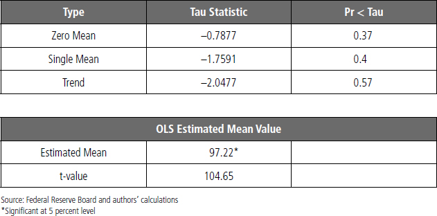
TABLE 14.13 Business Cycles and the U.S. Dollar

ECONOMIC POLICY: IMPACT OF FISCAL POLICY AND THE EVOLUTION OF THE U.S. ECONOMY

Looking forward, analysts will be challenged in their application of both economics and time series techniques when tracking and predicting the impact of significant changes in recent monetary and fiscal policy. They will need to recognize the magnitude and the unusual nature of our monetary and fiscal policy. Moreover, due to the overconfidence bias, forecasts of policy effectiveness for both fiscal and monetary policy have been too optimistic relative to actual outcomes. As mentioned, forecasts of the effectiveness of the 2009 fiscal stimulus and the first-time homebuyers' credit did not deliver.

Will our economic/statistical model of the impact of entitlement spending and debt-to-GDP ratios on the economy be wrong in a similar way? If our estimate of 2.75 percent trend growth is really the path of the future, will the clash of fiscal spending promises and continued monetary ease prove inconsistent with low inflation and interest rates? In addition, what happens if the long-term cycles of interest rates tend to move upward, as interest rates did in fact rise at the beginning of the post–World War II period, and as a result large fiscal deficits will be continuingly financed at higher nominal interest rates? Will there be a temptation to resort to inflation-financed federal deficits in the future? Should we also expect higher future taxes to pay for government spending? While we may be uncertain on how the economy will evolve, we know that something will change in the patterns of growth, inflation, interest rates, and the dollar we have evaluated so far. We cannot evaluate the patterns here, but let us take a look at the context of fiscal issues at least to provide a research agenda for the future.

Large and Persistent Deficits: A Brave New World of Fiscal Policy

As apparent in Figure 14.31, there has been a clear shift in the position of fiscal policy today compared to prior years and prior economic recoveries. Yet conventional measures of the fiscal deficit have misrepresented the true federal budget situation for more than 40 years. The unfunded liabilities of the entitlement programs reflect a commitment to spend in the future without any set-aside out of current revenues (see Figure 14.32).

As a result, the current federal budget appears to be much closer to balance since the unfunded liabilities are not accounted for in today's budget calculations. By not accounting for these liabilities, the public budget calculations for the past 40 years seriously overstated the positive position of federal, state, and local budgets within the U.S. economy. Only in recent years have taxpayers learned the true state of fiscal deficits as the retirement and healthcare bills begin to accumulate. As illustrated in Figure 14.33, estimates by the Congressional Budget Office indicate that the burden of these unfunded liabilities will alter fiscal policy expectations.¹⁵ These bills represent the risk of higher taxes, reduced after-tax incomes, and the potential for a lower standard of living for taxpayers than they had anticipated. The federal government might have to resort to central bank financing of the deficit to pay its bills. This would increase the risk of higher inflation, higher interest rates, and lower real growth and job gains in the future. This fiscal policy framework certainly alters the decision-making calculus for investors, savers, and business decision makers as they evaluate the path of growth, inflation, and interest rates going forward. Moreover, the time horizon for federal tax and spending policy has shortened dramatically in recent years with increased partisanship in Washington. As a final note, the pattern of mandatory outlays was tested for mean reversion, and the results exhibit a nonstationary pattern over, indicating no mean reversion in any sense.

FIGURE 14.31 U.S. Budget Gap

Source: Congressional Budget Office

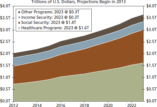
FIGURE 14.32 U.S. Fedral Government Mandatory Outlays

Source: Congressional Budget Office

FIGURE 14.33 U.S. Debt Held by the Public

Source: Congressional Budget Office

Budget Limits with 2.75 Percent Trend Economic Growth

Unfunded liabilities at any level of government will, in some combination, increase future taxes, lower direct government spending, and require greater debt financing, all problems evident during the past four years as government budgets have become tight in light of slower economic and revenue growth. At the federal level, the genesis of these problems began with Social Security, Medicare, Medicaid, and a number of stimulus programs under both Democratic and Republican administrations, underscoring their bipartisan nature. The longer-term fiscal outlook places the economy in a territory outside past experience, as the U.S. debt held by the public rises far above previous experience (see Figure 14.33).

In the short run, hard choices have been avoided by employing off-budget spending, emergency spending programs, mandates imposed on the private sector, and unrealistic budget and economic forecasts (the rosy scenario) that cover up the real nature of the fiscal problems. But not tackling these problems has had an economic impact on the real economy. The lack of the relationship between the reported fiscal deficit and the true budget imbalance has not addressed as well as the real choices needed to sustain a steady, or at least predictable, fiscal policy over time.

FIGURE 14.34 Prime Employment–Population Ratio

Source: U.S. Department of Labor

Auerbach, Gale, Orszag, and Potter build a case that current fiscal policies are far from addressing the federal government's real budget constraint.¹⁶ The demographic pressure on entitlement programs indicates that the ratio of working-age adults relative to those over 65 will decline in the decades ahead. In fact, the sharp drop in the employment-to-population ratio in recent years (see Figure 14.34) already signals a fiscal problem as fewer workers begin to support a larger entitlement-benefiting cohort. In addition, medical care technology continues to put upward pressure on medical spending, while current life expectancies exceed the expectations that existed when most of these entitlement programs were established. These forces are large and persistent. A widening gap between spending and revenues in the future will exist. In turn, investors and business decision makers will have to reevaluate their expectations regarding growth, inflation, and interest rates in such an environment where the federal budget will be unlikely to be balanced over the economic cycle and sudden changes in tax and spending policy could appear. Many policy adjustments will be needed, and they will influence the path of expected real after-tax incomes and profits. These policy options include some combination of tax increases, spending cuts, or higher inflation to reduce the real value of the federal debt.

THE LONG-TERM DEFICIT BIAS AND ITS ECONOMIC IMPLICATIONS

The theme of a deficit bias in fiscal policy is evident in the sovereign debt issues in Europe and the United States. For years, many decision makers have argued for a balanced budget, but disagreements between the political parties have made such a goal seemingly impossible. There is little evidence that policy follows a cyclical pattern trending toward balance.

How does this deficit bias come about? James Buchanan and Richard Wagner argue that the benefits of high purchases and low taxes are direct and evident, while the costs lower future purchases. Higher future taxes are indirect and less obvious. If voters do not recognize the extent of the costs or assume they will not pay these costs, then there is a tendency toward excessive deficits.¹⁷ This bias becomes even more accentuated when some voters perceive that they will not bear the tax burden of current and future spending. The euro crisis reflects the fundamental disconnect with patterns of current fiscal policy spending that could not be sustained over time, giving an ever-rising ratio of debt to GDP. The shock of the 2007 to 2009 recession made the debt-to-GDP imbalance an immediate crisis. Belated attempts to deal with the crisis resulted in sharp contractions in fiscal policy, a large decline in aggregate demand, major repercussions for capital and foreign exchange markets, and the potential for government default.

The euro experience follows a long history of financial crises that illustrate transitions from an unsustainable fiscal deficit position are rarely smooth, especially when the markets recognize that such a debt position is unsustainable. For example, we have witnessed a default in the case of Greece in recent years, or periods of sharply lower real exchange rates, increased inflation, and recessions, such as the case in Mexico. These crises disrupt capital markets, lower real investment, and reduce real economic growth.

Interest Rates Trend Reversal: Test to Come Ahead

For the United States, one path to a fiscal crisis is to not recognize that the trend growth for the country is closer to 2.75 percent in the near term than to the 4 percent that some forecasters estimate for the next two years or to sustain the belief that long-run trend growth is more like 3 to 3.5 percent (see Figure 14.35). Unfortunately, we are already seeing this disconnect in regard to pension and healthcare benefits promised over the past 40 years by federal, state, and local governments. These promises were made with expectations of growth stronger than we are currently experiencing and stronger than we anticipate going forward. Simply stated, based on current projections of economic and job growth, there is not likely to be enough tax revenue to pay the entitlement bills. When private and public investors recognize this weaker trend growth, they will begin to migrate away from U.S. Treasuries at current interest rates and the current exchange rate.

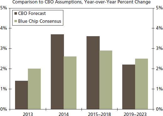
FIGURE 14.35 Real GDP Growth Estimates

Source: Blue Chip and Congressional Budget Office

This process may already be starting. The Bank of Japan has decided to follow Prime Minister Abe's program to ease monetary policy and promote an increase in inflation. In this case, the implication is that the yen would depreciate against the dollar. Yet a policy of monetary ease would also indicate a decreased interest by the Bank of Japan to buy Treasury debt. With Japan as one of three dominant buyers of Treasury debt (along with China and the Fed), Japan's decision would put some upward pressure on U.S. interest rates even while the size of Treasury debt issuance remains large. As in many markets, when traders and investors in China and the Cayman Islands sense that the direction of the bond market has changed, market rates will likely rise much faster than generally has been incorporated in current forecasts.

Credit Imbalance: The U.S. Treasury Market

Persistent, large future federal deficits, as illustrated in Figure 14.36, create significant uncertainties in financial markets. Will continued large federal deficits find sufficient demand at current interest rates, dollar exchange rates, and levels of inflation? How much will large federal financing squeeze out private sector investment? Something has to give, especially given the dominant role played by central bank Treasury-buying policies in Japan, China, and, ultimately, by Federal Reserve in the United States. Since these institutions are not motivated by profits but rather by concerns about exchange rate stability and/or unemployment, policy can change the demand for U.S. Treasury debt at a moment's notice, and for non–market-related factors.

FIGURE 14.36 U.S. Budget Gap

Source: Congressional Budget Office and U.S. Department of the Treasury

On the supply side of the Treasury debt market, consider that the model for fiscal policy today is for permanent deficits that must be financed. It is likely that household and business behavior would be different from under the traditional model. Since this model is different from what is commonly assumed, this behavior will likely evolve into another kind of economic outcome than what some have projected.

First, the economic impact of fiscal deficits that are perceived to be permanent and unsustainable will be different from the impact of deficits that are temporary and self-correcting. Permanent deficits must be financed by taxes/debt finance and possibly rising inflation over time. In addition, when deficits are perceived to be unsustainable, the risk is that future taxes will rise, debt finance will grow, and inflation has a strong upside bias. Higher future taxes cause greater caution among taxpayers who anticipate that higher future taxes will reduce their after-tax disposable income. Greater future debt finance increases the probability of higher taxes and/or higher inflation. Finally, permanent, unsustainable future deficits prevent the use of traditional fiscal policy models based on the customary assumption of temporary and self-correcting deficits. The framework of fiscal policy has changed, and the anchoring bias of basing current economic estimates on outdated models is very obvious today.

Second, current deficits finance current consumption. This also is a significant change from the past, when deficit finance focused on public infrastructure, such as highways. Those past deficits added to the nation's physical capital and to the potential improvement in long-run growth of the economy. Financing current consumption through transfer payments such as Social Security and Medicare supports current consumption, of course, but detract from the capital needed for long-run growth. These unfunded liabilities—entitlements—allowed the U.S. economy to exhibit above-average consumption in recent years, which was above the pace of consumption consistent with income gains. Those deficits allowed the U.S. economy to appear to be doing better than it really was. The U.S. economy is living on borrowed time and reducing the wealth of future generations either through higher future taxes or inflation to pay the debt.

Finally, time shifting in taxation and deficit finance provides a bias for more spending today. Current fiscal policy—government-financed consumption—favors today's voters at the cost of the young and future generations who are not yet voters. This helps explain the unfunded liabilities of entitlements at the federal, state, and local levels. These liabilities reinforce the risk to current workers, who are not entitlement recipients, of higher taxes/debt finance/higher inflation over time while limiting their spending today when deficits are perceived to be permanent and unsustainable. When faced with the choice of “pay me now” or “have someone else pay later,” current entitlement recipients and policy makers shift the burden to future taxpayers (nonvoters).

The altered model of fiscal policy, permanent large deficits as illustrated above in Figure 14.36, helps to show why current spending did not generate the economic growth or jobs that were promised. The lack of stimulus follow-through on the demand side also helps to show why interest rates have not risen as some anticipated, although the impact of the supply of credit from China and Japan as foreign buyers of U.S. Treasuries (Figure 14.37), and the Federal Reserve as well helps explain the continued low interest rates. Some analysts have argued that the failure to see higher interest rates indicates that deficit financing did not have a negative impact and therefore that federal, state, and local governments can spend even more money. However, that argument only takes a pure demand-side view of the credit market. It overlooks the impact of the supply of credit from China and other nations, the depressing effect on current consumption and higher saving, and/or the deleveraging of current taxpayers who are discounting the impact of higher future taxes on their disposable incomes. Deficits without tears?

FIGURE 14.37 Top Holders of U.S. Treasuries

Source: Congressional Budget Office and U.S. Department of the Treasury

Fiscal deficits have delivered a stretch of subpar economic growth of 2 percent over the past three years as well as two years of job growth of 180,000 per month on average for each year, a disappointing number. The price of temporary programs, policy uncertainty, and model uncertainty has been subpar economic growth. Moreover, federal debts are paid in a fiat currency, the dollar, the supply of which the Fed has increased dramatically over the past five years. This increases the risk of higher inflation sometime in the future.

SUMMARY

The relationship between economic and financial variables evolves over time. In addition, the behavior of individual data series also changes with the passage of time. There is a tendency either to believe in the past findings (e.g., that GDP growth rate and unemployment rate, Okun's law, has a statistically significant relationship) or to make an assumption about the behavior of an individual variable (e.g., inflation rate is mean reversion) in decision making. Our approach is to test/quantify statistical relationships between variables of interest using econometric techniques and the most recent dataset instead of making assumptions of about the relationships.

Statistical software enables analysts to use major econometric techniques to characterize a variable and/or to quantify a statistical relationship between variables of interest. Without learning the tedious math, analysts can employ these statistical tools to perform the required tests.

Users must be aware, however, that statistical software produces results without considering the type of input dataset. It is an analyst's job to make sure the input dataset fulfills economic/financial theory and matches the statistical properties of the underlying tests.

The challenges for analysts going forward require that we anticipate change in our economic and financial benchmarks and model those changes. We await the results.