CHAPTER 10

A Single-Equation Approach to Model-Based Forecasting

Model-based forecasting approaches are essential elements in the process of effective decision making. One major benefit of using these forecasting approaches is that the model can serve as a baseline for adjusting economic guidance for risk assessment, and a model's forecasting performance can be monitored over time to compare expected versus actual outcomes. In addition, a model that is not performing as expected can be revised and rebuilt to improve guidance to decision makers. Decision makers utilize models to generate both long-term and short-term forecasts. The focus of this chapter, however, is on short-term forecasting.¹ We discuss different methods to build forecasting models and describe which method may be appropriate for a forecaster depending on the forecasting objective and on the available data set.

This chapter focuses on single-equation, univariate, forecasting. A univariate model contains one dependent variable and one or more predictors (independent variables). Within a univariate forecasting framework, we discuss two approaches: unconditional and conditional forecasting. With the unconditional forecasting model, we do not need out-of-sample values of predictors to generate an out-of-sample forecast. Conditional forecasting, in contrast, implies that the forecasted values of the dependent variable are conditioned on the predictors' values. Another major difference between unconditional and conditional forecasting is that sometimes unconditional forecasting includes only lags of the dependent variable and error terms as right-hand-side variables. The conditional forecasting models, however, include additional variables as predictors.

The conditional forecasting approach is divided into two broader categories: (1) when a dependent variable is traditional in form (i.e., the dependent variable can contain any numerical value), and (2) when a dependent variable is nontraditional in the sense that it is a dummy variable (binary variable) and contains only two values, zero and one. The division between these two conditional forecasting approaches reflects different estimation techniques. A model with a dummy-dependent variable is sometimes referred to as a logit or probit model and these models are commonly used to predict the probability of an economic event.

In this chapter, we provide a detailed discussion of unconditional, conditional, and Probit forecasting approaches. We suggest guidelines for the analyst when choosing between the unconditional and the conditional forecasting approach as well provide SAS codes to help generate forecasts.

THE UNCONDITIONAL (ATHEORETICAL) APPROACH

Typically, a forecaster can utilize economic/financial theory to build a model. However, sometimes economic/financial theory is unable to provide guidelines for forecasting for two main reasons: (1) the reliability of an economic theory is questionable (at least in the short-run) and (2) the potential predictors (based on the economic theory) are not available at the desired frequency.

Recently, the Great Recession rendered less reliable several economic theories (at least in the short-run), with one example being Okun's law.² Okun's law posits a relationship between the gross domestic product (GDP) growth rate and the unemployment rate. However, the recovery period from the Great Recession does not replicate this relationship, as GDP entered into expansionary territory, surpassing its pre-recession level while the unemployment rate remained stuck at elevated levels for a significant amount of time. This scenario makes a forecaster wonder whether he or she should utilize the GDP growth rate to forecast unemployment rates over the short-run.

Economic/financial theory is also unable to help a forecaster when the desired forecasting frequency of the dependent variable is different from the potential predictors that economic/financial theory suggests are the most appropriate variables. For example, if we wanted to forecast the daily closing price of the Standard & Poor's (S&P) 500 index, it will be hard to find an explanatory variable that is also reported at a daily frequency. Therefore, we may not be able to include valuable predictors in our forecasting model. In this case, the unconditional forecasting approach is a useful tool.

The unconditional forecasting approach includes both the lags of the dependent variable and stochastic error terms as right-hand-side variables. Since there is no economic/financial theory behind the unconditional forecasting approach, it is also known as an atheoretical forecasting approach. The lags of the dependent variable that are used as right-hand-side variables are called autoregressive (AR), and the number of lags is denoted by p. Hence, the notation AR (p) shows the number of lagged dependent variables that are used as right-hand-side variables. Let us assume that y_t(y_t-1 and y_t-2)as right-hand-side variables, then we say y_t, follows AR (2) process, as shown in equation 10.1.

where

ε_t = white noise error term

β = parameters to be estimated

The general form of an AR (p) process, which includes up to p lags of the y_t as right-hand-side variables, is shown in equation 10.2.

Put simply, if y_t follows an AR (p) process, it implies that only the p lags of y_t are needed to generate a forecasted value of the y_t series.

The second possibility when forecasting is to use the stochastic error terms as the only right-hand-side variables. In this case, y_t follows a moving average (MA) process. The number of lag values of the error terms are defined by q, and MA (q) states the y_t series follows the MA process using up to q lags of the error term. Equation 10.3 implies that y_t is generated by the MA (q) process, and ϑ is a constant term.

The third possibility is that both AR and MA processes are used in predicting y_t. In this case, an ARMA (p, q) model is needed to forecast y_t.³ Equation 10.4 is an example of an ARMA (1, 1) model where the first lagged value of y_t as well as lag-1 of error term (ε_t) are utilized to predict y_t, where θ is a constant.

Most time series data involve a nonstationary characteristic so we need to identify the order of integration, I (d), whether the series is nonstationary or not. We combine the process to identify the orders of AR (p), MA (q), and I (d), which is known as ARIMA (autoregressive integrated moving average).⁴ An ARIMA (p, d, q) model can be built to forecast y_t.

The Box-Jenkins Forecasting Methodology

How do we determine the order of an ARIMA (p, d, q) model? What are the appropriate values for p, d, and q? The answer to this question is provided by Box and Jenkins (1976) and is known as the Box-Jenkins (B-J) methodology.⁵ The technical name of the B-J methodology is ARIMA modeling. The B-J approach consists of four steps: (1) identification, (2) estimation, (3) diagnostic checking, and (4) forecasting.

Step 1: Identification

The first step in the B-J methodology is to identify the order of the ARIMA model—the values for the p, d, and q. Traditionally, the plots of autocorrelation functions (ACFs) and partial autocorrelation functions (PACFs) were utilized to determine the value of p, d, and q.⁶ But SAS software provides a user-friendly method to identify the order of ARIMA (p, d, q), known as the SCAN method, for the smallest canonical correlation approach. SAS identifies the appropriate order of ARMA/ARIMA for a given time series.⁷ We suggest using the SCAN approach because it uses a broader range of p, d, and q to determine the appropriate values of ARIMA (p, d, q) model.

Step 2: Estimation

Once an analyst identifies the order of the ARIMA (p, d, q) model, the next step is to estimate the identified model. Statistical software can be used to estimate the model, which we demonstrate in coming sections.

Step 3: Diagnostic Checking

The next step is to check the model's goodness of fit. One standard way to do so is to examine whether the estimated residuals from the chosen model are white noise. The idea behind the white-noise testing is that if the estimated residuals are white noise, then no additional information outside of the model should be included. If the estimated residuals are white noise, then the estimated model can be used to forecast the target variable. However, if the estimated residuals are not white noise, it implies that there is a residual presence of autocorrelation, and we will have to return to the first step and again identify the ARIMA (p, d, q) model to eliminate the autocorrelation, repeating steps 2 and 3 as well.

Step 4: Forecasting

The last step of the B-J approach is forecasting of the target variable. That is, after estimating the chosen model, we utilize the estimated coefficients to generate forecast values for the target variable.

Overall, the B-J approach is very useful for short-term forecasting (up to a few months ahead), not long-term forecasting. Because the economy contains several moving elements over time, the analyst will find it useful to include predictors to capture the state of the economy in a forecasting model, especially for medium- and long-term forecasting.

Application of the Box-Jenkins Methodology

As an example, we will apply B-J methodology on a data series of the number of initial claims filed for unemployment, released as a weekly series by the U.S. Department of Labor (DoL).⁸ The initial jobless claims series provides an early look at the state of the labor market because other labor market indicators such as nonfarm payrolls and the unemployment rate are released on a monthly basis. While initial jobless claims data can be used to predict labor market indicators, forecasting the initial claims series itself is not easy. One major reason for that is that there are not many economic indicators available on a weekly basis that can be utilized in the forecasting model. The B-J forecasting approach, therefore, would be a practical option given the weekly frequency of the initial jobless claims data series.

Figure 10.1 shows the number of initial unemployment insurance claims (in thousands) filed in a given week. In analyzing this data, the first step is to apply a unit root test, such as the augmented Dickey-Fuller (ADF) test, on the target series to determine whether the series is stationary. In other words, find the order of ‘d’ for the initial claims series. The analyst can then utilize the SCAN approach to determine the order of ARMA (p, q).⁹

FIGURE 10.1 Number of Initial Claims Filed for Unemployment Insurance

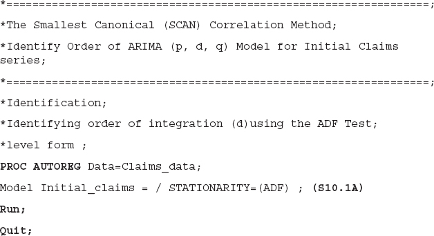
TABLE 10.1A ADF Test Results Using Level Form of Initial Claims

SAS code S10.1A is used to perform the ADF test on the level form of the initial claims data series and the results based on the code are reported in Table 10.1A. The middle part of the table shows the ADF test results. The null hypothesis of the ADF test is that the series is nonstationary, and the alternative hypothesis is that the series is stationary. If a series is stationary at level form, the ‘d’ for that series is zero (d=0). If the first difference of a series is stationary, then the ‘d’ would be 1 (d=1). From Table 10.1A, we cannot reject the null hypothesis of nonstationary for initial claims at a 5 percent level of significance because the p-values (Pr < Rho, Pr < Tau, and Pr > F) are greater than 0.05.

The first difference form of the initial claims data is tested for stationary behavior using SAS code S10.1B and the results are reported in Table 10.1B. At a 5 percent level of significance, we reject the null hypothesis of nonstationary behavior and suggest that the first difference of the initial claims data series is stationary, and ‘d=1.’ We will utilize the first difference form of the initial claims data in the SCAN approach.

Using SAS code S10.2, the SCAN approach is performed on the initial claims series (first difference). The results are reported in Table 10.2.¹⁰ In the second line of the SAS code, Initial_claims(1),(1) indicates the first difference of the initial claims series. It is important to note that since we already selected the order of ‘d’ through ADF testing, the label ‘p+d’ in Table 10.2 will provide order for ‘p’ only, not for ‘d.’ The SCAN option provides three tentative and different orders for ‘p’ and ‘q,’ which are MA (2), ARMA (2, 1) and AR (4). The question arises: Which ARMA order an analyst should select for forecasting? A simple answer is that we estimate three different models using these three orders and test the estimated residuals for autocorrelations from each model. Then we then select the one that produces white noise–estimated residuals. Interestingly, in the present case, all three orders produced white noise residuals.¹¹ In these kinds of scenarios, an analyst should utilize other available tools to select a model. The information criteria can be used to choose a model among its competitors. We employ the Schwarz information criterion (SIC) to select the model. We run three different ARIMA models using three different orders and the MA (2) model produces the smallest SIC values; therefore, that is our preferred model for forecasting.¹²

TABLE 10.1B ADF Test Results Using Difference Form of Initial Claims

TABLE 10.2 SCAN Results Finding Tentative Order of ARMA (p, q)

Once an analyst has selected a particular ARIMA order for a given series—in this case we select p=0, d=1 and q=2—the next step is to test the reliability of the selected model. The standard approach is to estimate the model and test the estimated residuals for autocorrelation. If the estimated residuals show no autocorrelation, we will use the selected model for forecasting.

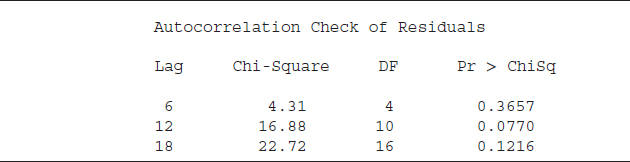
SAS code S10.3 performs an autocorrelation test (Chi-square) on the estimated residuals, and the results are reported in Table 10.3. The null hypothesis of the Chi-square test is that there is no autocorrelation (or white noise) and the alternative hypothesis is that there is autocorrelation. The first column, labeled “Lag,” indicates how many lags we include in the test equation (up to 18 lags in this test).¹³ The Chi-square statistic and the degrees of freedom (DF) are presented in the second and third columns, respectively. The p-values (under the label “Pr > ChiSq”) are greater than 0.05 for all lag order, implying that we cannot reject the null hypothesis of white noise and the estimated residuals are white noise. Put simply, the identified model for initial claims (p=0, d=1, and q=2) passed the diagnostic test. The next step is forecasting initial claims using the identified model.

TABLE 10.3 Autocorrelation Check of Estimated Residuals

SAS code S10.4 estimates and generates forecasts for the initial claims series. The fourth line of the code starts with Forecast, which is a SAS keyword to generate the forecast for the dependent variable. The option, lead=8, is asking SAS to provide forecasts for the next eight periods. interval=weekly indicates the weekly frequency of the dataset, and id=date shows that the datevariable is utilized as ID. The output is saved in the file name forecast_Claims. We plot the actual values and forecasted values for the initial claims series in Figure 10.2. From the figure, upper and lower lines represent the 95 percent confidence interval (the upper and lower forecast bands). Overall, the fitted values are consistent with the actual values. Note that the model accurately predicted the spikes in claims in 2011 and 2012.

In conclusion, the B-J procedure and SAS codes provided in this chapter can be utilized to forecast financial and economic variables. At this point, we expect an analyst to be familiar with the notion behind the B-J approach as well as its application in SAS.

FIGURE 10.2 Initial Claims Forecast and 95 Percent Confidence Interval

THE CONDITIONAL (THEORETICAL) APPROACH

Several economic and financial theories provide guidelines that can be utilized to build a forecasting model. One example, the Taylor rule, suggests inflation expectations, and the output gap would describe the likely path of short-term interest rates, in particular the federal funds rate.¹⁴ Therefore, the analyst can build a forecasting model for the short-term interest rate using guidelines from the Taylor rule. The idea here is that with the help of an economic/financial theory, we can build an econometric model and forecast the dependent variable based on predictors. While a forecasting model can contain two or more dependent variables with two or more predictors, the focus of this chapter is on single-equation forecasting. Chapter 11 discusses forecasting models with two or more dependent variables.¹⁵

The fundamental idea behind a single-equation forecasting approach is the utilization of economic and financial theory to identify the dependent variable and its predictors. Econometric techniques can then be utilized to estimate coefficients of the model, and an out-of-sample forecast can be generated with the help of the estimated coefficients and out-of-sample values of predictors.

One requirement of the single-equation approach, however, is that we must insert out-of-sample values of the predictor(s) for the desired forecast horizon in the model. Because of this, the approach is also known as conditional forecasting since out-of-sample forecasts of a dependent variable are conditioned on the predictors' future values. For example, an analyst can build a forecasting model using the Taylor rule with the model containing the Fed funds target rate as the dependent variable and the consumer price index (CPI) and GDP as predictors. The analyst must have future (out-of-sample) values for the CPI and GDP to generate an out-of-sample forecast for the Fed funds target rate. There are different ways to obtain future values of the predictors. ARIMA models can be utilized to generate out-of-sample forecasts of predictors, for example.¹⁶ Another way to obtain out-of-sample values of predictors is to assume different economic scenarios for both series. Using CPI and GDP as an example, these difference scenarios might include (1) higher inflation with lower GDP growth rates, (2) subpar inflation and GDP growth rates, and (3) stronger GDP and inflation rates. This approach, which is also known as scenario-based analysis, is widely used in both public and private decision making.

The major benefit of scenario-based analysis is that, in the present case, different economic scenarios of inflation and GDP growth rates would provide corresponding different paths of the Fed funds rate. These varying scenarios will help decision makers in budget planning and investment decisions.

A Case Study of the Taylor Rule

We forecast the Fed funds target rate using the conditional (single-equation) forecasting approach. The original Taylor rule suggests that the nominal, short-term interest rate should respond to changes in inflation and output. Therefore, by utilizing future values of inflation and output growth rates, an analyst can forecast the Fed funds rate. One modification of the Taylor rule is that the future values of the Fed funds target rate also depends on the current level of the Fed funds rate.¹⁷ That said, we estimate a modified Taylor rule to forecast the Fed funds target rate, using CPI as a proxy for inflation and the GDP growth rate as a proxy for output. We estimate equation 10.5:

The ε_t is an error term. The level of the Fed funds rate, the compound annualized quarterly growth rate of the real GDP, and the year-over-year (YoY) percentage change of the CPI is included in the regression equation. Since inflation expectations are a key determinant of short-term interest rates, we use the YoY form of the CPI with the current level of Fed funds to capture the inflation expectations effect. The 1984:Q1 to 2012:Q4 period is used for estimation purposes, and Fed funds is forecasted for the 2013:Q1 to 2014:Q4 period (eight quarters ahead).

SAS code S10.5 is utilized to estimate equation 10.5. PROC MODEL is employed because it is a useful procedure for conditional forecasting.¹⁸ The second line of the code shows the estimation equation, where the Fed funds is the dependent variable and CPI, GDP, and the lag of the Fed funds are right-hand-side variables. The ao is an intercept and a1 to a3 are the coefficients to be estimated. In the third line, Fit is a SAS keyword that instructs SAS to estimate the equation for the Fed funds rate. Solve is a SAS keyword to generate forecasts for the variable of interest. The option out=FF_Forecast will save forecasted values of Fed funds rate in the data file named FF_Forecast, and the forecast option instructs SAS to generate a forecast for the Fed funds rate. Outvars is a SAS keyword that instructs SAS to include a specified variable in the output. That is, we ask SAS through the Outvars option to include variable date in the output file, which is FF_Forecast. The reason to include date variable in the output file is that the output file does not have a date variable, and we cannot tell which value is for what time period.

The results based on code S10.5 are reported in Table 10.4. The first part of the table shows summary statistics. The R² is very high and may suggest that the model fit is very good. The bottom part of the table exhibits individual variable statistics, such as the estimated coefficients and their corresponding t-values. The last column provides p-values for each estimated coefficient including the intercept. Based on the p-values, at 5 percent level of significant, all right-hand-side variables except CPI are statistically significant. Since we built equation 10.5 (our regression equation to generate the forecast) on economic theory, we will keep CPI in the final equation. One possible reason for the statistically insignificant coefficient of the CPI is that during the last couple of decades, inflation was not a significant factor in determining interest rate because inflation rates stayed around the target rate set by the Federal Open Market Committee (FOMC).

After estimating the regression equation for the Fed funds rate, we want to generate a forecast. Two key components to generating a forecast are the estimated coefficients and the out-of-sample values of the predictors (CPI and GDP). From Table 10.4, we do have an estimated coefficient for the CPI and GDP, but we still need the out-of-sample values of the predictors. One option is to use a forecast from a reliable source (either public or private sector) as out-of-sample values for GDP and CPI.¹⁹ We utilize Wells Fargo Economics Group's forecasts for GDP and CPI and as out-of-sample values to generate the forecast for Fed funds rate for the 2013:Q1 to 2014:Q4 period.

TABLE 10.4 PROC MODEL Results for the Estimated Taylor Rule

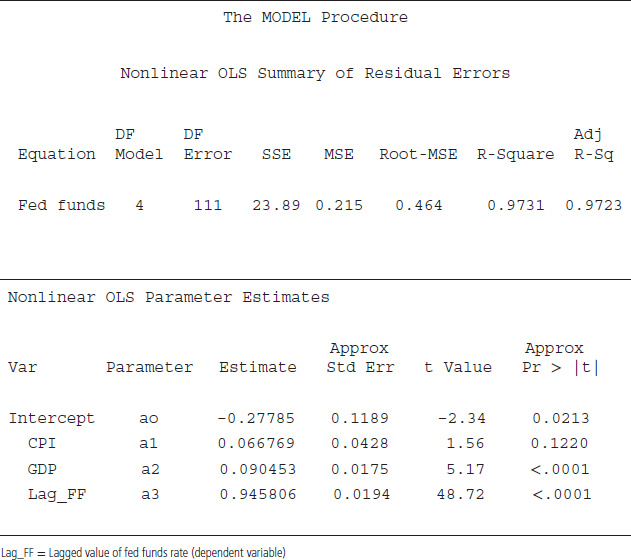
Table 10.5 provides conditional out-of-sample forecasts of the Fed funds rate with the out-of-sample values of GDP and CPI. The Fed funds forecasts are conditional because if we change values of GDP and/or CPI then the forecasted Fed funds rate will also change. In this case, the out-of-sample values of the CPI are around the FOMC inflation target of 2 percent and GDP shows trend growth rates around 2 to 2.5 percent. Therefore, both predictors exhibit normal or trend growth. For that reason, we will choose this case to be the base-case scenario for path of the Fed funds rate.

The plot of the actual and forecasted Fed funds rate is shown in Figure 10.3. Given that the CPI values are around the FOMC inflation target and GDP growth is weak, the Fed funds rate moves upward very slowly, at 0.63 percent by the end of 2014. In a scenario of low inflation and low GDP growth rate, the FOMC is likely to keep the fed funds rate lower, with the intention of stimulating the economy.

TABLE 10.5 Base-Case Scenario: Forecast for Federal Funds Rate Conditioned on CPI and GDP Growth

FIGURE 10.3 Base-Case Scenario: Forecast for Federal Funds Rate Conditioned on CPI and GDP Growth

The major benefit of the conditional forecasting approach is that the analyst can generate different paths (scenarios) of the conditioned on different paths of the predictors. In the scenario just given, the Fed funds target rate forecast is conditioned on normal, or perhaps subpar, growth rates of GDP and CPI. However, what would be a likely path for Fed funds rate if the economy experiences a different scenario?

TABLE 10.6 Strong GDP Growth Rate Scenario: Forecast for Federal Funds Rate Conditioned on CPI and GDP Growth

What About Strong Growth?

We explore the possibility of stronger GDP growth rates in Table 10.6.²⁰ In addition, we added 2 percent into the base-case GDP growth rates (out-of-sample values) and kept the CPI values the same. We stress here the important question: What would be the likely move of the FOMC (in terms of Fed funds decisions) if the economy shows a stronger GDP growth rate? From Table 10.6, we see that the Fed funds rate increases at a much faster rate, being about three times higher than the base-case scenario by the end of 2014. The plot of actual and forecasted Fed funds rates is exhibited in Figure 10.4. The plot shows the forecasted Fed funds rate as a steep curve and reaches around 2 percent (1.83 percent) by the end of 2014. That said, private sector borrowing costs may increase at a faster rate during a stronger GDP growth rate environment compared to the subpar economic growth scenario illustrated in Table 10.5.

In conclusion, the single-equation conditional forecasting approach is very useful for decision makers to generate different likely paths of economic and financial variables and to make budget/investment planning decisions.

FIGURE 10.4 Strong GDP Growth Rate Scenario: Forecast for Federal Funds Rate Conditioned on CPI and GDP Growth

RECESION FORECAST USING A PROBIT MODEL

In the previous two sections, we discussed unconditional (atheoretical) and conditional (theoretical) forecasting approaches within a single-equation regression framework. The major difference between the two approaches is that the unconditional forecasting approach does not include any additional predictors and uses statistical tools to characterize and forecast the variable of interest. Conditional forecasting, in contrast, utilizes predictors, usually identified with the help of economic/financial theory, in a regression analysis. Furthermore, out-of-sample forecasts of the target variable are conditioned on the predictors' values.

Common, however, between the two approaches is the functional form of the target variable. Sometimes a dependent variable may be nontraditional, in the sense that it contains a specific set of values, such as zero or one. This is known as a dummy-dependent variable model.²¹ A regression analysis involving a dummy-dependent variable is known as a binary dependent variable regression. In the case of a binary regression, traditional econometric techniques, such as ordinary least squares (OLS), do not provide reliable results. This is because a binary regression is required to predict outcomes in a specific range such that the predicted values of the dependent variable stay in the zero to one range. The Probit model provides reliable results in the case of a dummy dependent variable regression analysis.²²

Probit models are used in both public and private decision making to predict the probability of an event. One application of a Probit model is to predict the probability of a recession. Several studies have employed the Probit approach to predict recession probability for the U.S. economy; see Silvia, Bullard, and Lai (2008) for more details.²³ Recently, a study by Vitner et al. (2012) proposed Probit models for all 50 states.²⁴ It is important to note that whether we are interested in predicting the recession probability for the U.S. (or any other country) economy or for a state, the fundamentals of a Probit model are the same. First, we need to create a dummy variable that is equal to one if the underlying economy is in recession and zero otherwise. Silvia et al. (2008) provided a detailed methodology to identify predictors for a Probit model to predict recession probability for the U.S. economy. This methodology can be replicated in the application to any other economy. We follow the Silvia et al. (2008) Probit model as a case study.

Application of the Probit Model

The first step to build a Probit model to predict the probability of a recession is to generate a dummy variable, which will be the dependent variable of the model. The dummy variable in our model equals one if the U.S. economy is in recession and zero otherwise. The National Bureau of Economic Research (NBER) provides official dates of peaks (the beginning of a recession) and troughs (the end of a recession) for the U.S. economy, which can be employed to create a dummy variable.²⁵ Specifically, the dummy variable will be equal to one for the months between peaks and troughs, and therefore in recession, and zero for the other months in the sample period.

The next step is to find predictors for the Probit model. Using the Silvia et al. (2008) model, we employ these three predictors: (1) the S&P 500 index; (2) the index of leading indicators, also known as LEI; and (3) the Chicago PMI employment index.

Once we generate the dummy variable and identify predictors for the Probit model, the final step is to determine the forecast horizon. How far in the future do we want to forecast? For instance, Silvia et al. (2008) forecasted the probability of a recession during the next six months. We follow that same forecast horizon. The forecast horizon would indicate the functional form (current versus lags) of the dependent variable and the predictors. A six-month lag of the dummy variable instead of the current value is included in the test equation. In addition, the current form of the predictors is used in the model. There are two major reasons we use a six-month lag of the dependent variable with current values of the predictors. First, the regression output from the Probit model allows an analyst to measure the historical strength of the predictors to forecast six-month-out recession probability. Silvia at el. (2008) utilized a pseudo R² to judge the in-sample fit of the model. The second benefit of including six-month lags of the dependent variable is that to make a six-month-ahead forecast, we can utilize the current-month values of the predictors, which are available at the time of forecasting. The logistic equation 10.6 is estimated:

where

Y_t+6 = dummy dependent variable (six-month lead) that equals 1 if the U.S. economy is in recession and zero otherwise

α, β₁, β₂, β₃ = parameters to be estimated

LEI, SP500, and PMI_EMP (Chicago PMI employment index) = predictors

ε_t = error term

Since the dependent variable is a dummy (1, 0) and the predicted probabilities must stay between the zero and one range, equation 10.7 would keep predicted probabilities in the required range. Equation 10.7 is a typical Probit model estimation equation. The left side of the equation indicates the probability of a recession is given on the values of predictors, which are LEI, SP500, and PMI_Emp. The right-hand side of the equation consists of estimated coefficients along with the predictors.²⁶

where

Y = 1 implies recession

LEI, SP500, and PMI_Emp = predictors

Φ = cumulative standard normal distribution function that keeps the predicted probability in the zero to 1 range

So far we have discussed Probit modeling and key elements of a Probit model, such as the requirement to create a dummy dependent variable, the need to identify predictors of the model, and the identification of the forecast horizon. The next step is for SAS to generate a recession probability for next six months.

SAS code S10.6 is employed to estimate the six-month-ahead recession probability for the U.S. economy.²⁷ The PROC LOGISTIC command is utilized, and the data file data_Probit contains all variables of interest. The SAS keyword descending orders the dependent variable according to the objective of the study. That is, in a binary choice model such as ours where nonevent (no recession) equals zero and event (recession) has a value of 1, PROC LOGISTIC, by default, estimates the probability for a lower value, which is a nonevent (no recession). However, we are interested in the probability of a recession (probability of an event's occurrence), and the keyword descending instructs SAS to generate the probability of a recession conditioned on the predictors. The dependent variable, NBER_6M, and predictors, LEI, SP500, and PMI_EMP, are listed in the second line of the code.

We utilized month-over-month percentage changes of all the predictors instead of the level form because the level form often shows nonstationary characteristics. The growth rate (difference) form usually follows stationary path. link=Probit is another SAS keyword, which instructs SAS to fit a Probit model. The third line of the code saves the model's output in a desired file; we created the Probit_output data file, which contains actual values of the predictors and the dependent variable. The keyword Pred=probability_value produces a recession probabilities series, and that series is also saved in the data file Probit_output.

In Figure 10.5, we plot the probability of a recession. Shaded areas in the figure are recessions determined by the NBER. We generate a graph for the quarterly series, using three-month averages as a quarterly value because there is a lot of noise in the monthly series (see Figure 10.6). The quarterly graph for recession probability is much smoother and shows that the model produced a significantly higher probability during all recessions since 1980. That is, the Probit model successfully predicted all recessions since 1980.

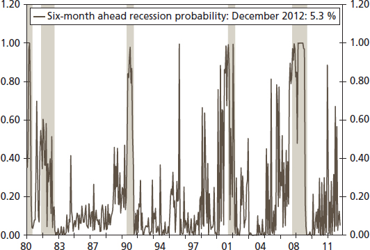
FIGURE 10.5 Recession Probability Using Monthly Data

FIGURE 10.6 Recession Probability: Quarterly Average

SUMMARY

In this chapter we provided different methods of forecasting within a single-equation framework. The first method, the ARIMA model, is a very useful forecasting tool for high-frequency variables, such as the S&P 500 index's daily closing price or weekly initial claims data. When there are not many predictors available to include in such a model, the ARIMA approach is useful because it does not require additional variables to build a forecasting model.

The second forecasting method discussed was the conditional/theoretical approach. In this case, there are several predictors available to include in a forecasting model. The benefit of this approach is that a forecaster can generate different forecasts of the target variable conditioned on different values of the predictors.

The third method the analyst can use to predict the probability of a recession is a Probit model. This approach is widely used in both public and private decision making.

The question arises: What method is more beneficial for an analyst? All three methods are useful, and the choice depends on the forecasting objective. For instance, because it would be very difficult to build a conditional forecasting model to predict the daily closing price of the S&P 500 index, and the practical approach is to utilize ARIMA models. Similarly, conditional forecasts of the Fed funds target rate for the next couple of years, using different economic growth and inflation scenarios, would be more useful than a forecast from an ARIMA model (since ARIMA model would provide just one likely path of the Fed funds target rate). Predicting recession probability conditioned on predictors is more appropriate than an ARIMA model because predictors will capture the underlying state of an economy, which would increase reliability of the Probit model.

In short, all three methods are useful at different times and in different circumstances. An analyst must be familiar with all of these forecasting approaches.