CHAPTER 6

Characterizing a Time Series Using SAS Software

Attempts to quantify the economic and financial relationships between variables with the help of econometric techniques extend back to the founding of the Econometric Society in 1930.¹ Over the past 20 years, the breadth of applications of time series analysis has expanded, with analysts relying extensively on real-world data and statistical software. These applications have extended far beyond the limited realm of traditional macroeconomics, and analysts who employ such methods extend far beyond the academic world. Much of the core economic and financial data utilized in applied econometric analysis is now available online and, in some cases, for a small cost. Furthermore, data often is available for use in a statistical analysis in a user-friendly format, such as Excel. Over the years, data collection methods have improved, increasing the scope of the data available.

Software that incorporates key econometric techniques has become an essential element of modern-day quantitative analysis. Such software produces statistical results in a few minutes, rather than hours, for routine techniques such as regression analysis. Until the late 1980s, it usually took researchers several days to estimate a regression. Researchers had to manually collect the data, format it to fit the needs of the statistical model, and finally calculate the results. While today's data processing is much quicker and relatively inexpensive, the risk is that researchers may be tempted to skip necessary steps in understanding the data, model, and results.

In this chapter, we specify the data (transform it if necessary) to properly test an economic hypothesis to illustrate key econometric techniques to test a hypothesis. We focus on using the econometric tools in SAS software and how to review SAS output.

TIPS FOR SAS USERS

One of the crucial elements of modern-day applied time series analysis, or any other applied quantitative analysis, is the econometric software. Statistical software is used at every level of applied research, from the basic level used by undergraduate students, to the advanced level used by policy makers, managers, and academics. Due to the flexibility of today's statistical software, an analyst may not need to learn the tedious math behind econometric techniques. However, the analyst still must be familiar with key econometric concepts, know how to employ econometric techniques in SAS software (or in any other statistical software), and know how to analyze the results produced by SAS.

SAS software is a powerful tool that offers a wide variety of econometric techniques. SAS is both a company and a widely known product around the world.² Originally, the acronym SAS stood for Statistical Analysis System; later SAS products became so diverse that the company officially dropped the full name and became simply SAS.

We employ SAS 9.3 in this book and in our workplace.³ SAS software offers a wide variety of software products, and we use Base SAS and SAS/ETS (Econometric and Time Series Analysis) at work.⁴ We further divide the SAS application processes into two broader steps: (1) the DATA step and (2) the econometric analysis, which we call the PROC step.⁵ The Base SAS helps us in the DATA step, and the PROC step is heavily based on the SAS/ETS products.

Whether an analyst wants to characterize a time series (e.g., estimation of a time trend, unit root test, etc.) or determine a statistical relationship between variables of interest (e.g., correlation, regression analysis, or Granger causality test), we follow this two-step process. The DATA step is similar to a foundation of a building, and the PROC step is the superstructure built up on this foundation.

Since data is the foundation of a time series analysis, we start with the DATA step. The first element of the DATA step is to import the dataset into the SAS system. Typically, an analyst has a dataset in an Excel spreadsheet, which needs to be brought into the SAS system to create a SAS dataset.⁶ After creating a SAS dataset, we can modify the dataset according to the objective of the study. For instance, after importing a dataset into SAS, we can convert the variables of interest into log-difference form from the level form.

The PROC step consists of econometric analysis (i.e., it employs econometric techniques to test the underlying hypothesis). For instance, an analyst wants to test money neutrality using the U.S. data. The first step, the DATA step, is to import a dataset consisting of the money supply (M2) and inflation rate (personal consumption expenditure [PCE] deflator). Since M2 usually is reported in billions of dollars while the PCE deflator is an index, there are two different scales for these two variables. For that reason, it is better to use a log-difference form of the variables, which is the DATA step. After converting both variables into a log-difference form, we can apply regression analysis to estimate the relationship between the money supply and inflation rate. The estimation part is the PROC step. Put simply, the DATA step properly specifies the dataset, and the PROC step handles the estimation process of any applied study.

THE DATA STEP

SAS has specific naming conventions for files and variables. A SAS name is user defined; that is, an analyst can choose the names for variables of interest and for the dataset. Whenever an analyst creates a SAS dataset, he or she must import data into SAS from an Excel or CSV file and assign a SAS name to the file.

The analyst also needs to choose SAS names for variables in the dataset. Rules for choosing a SAS name are flexible. Many SAS names can be as long as 32 characters, although some have a maximum length of 8 characters. The first character of a SAS name must be an English letter (A, B,C, . . ., Z) or underscore (_). Subsequent characters can be upper- or lower-case letters, numeric digits (0,1,2, . . .,9), or underscores. The few prohibitions on SAS names include spaces and special characters, such as the percent sign (%) or the at sign (@).⁷

Suppose we import data on the money supply and the inflation rate in a file with the SAS name of money_inflation. In a next step, we choose “M2” for money supply and “PCE_deflator” for inflation rate. Now the data file contains the variables M2 and PCE_deflator, both of which are in level form. If we wish to generate the log-difference form of M2 and PCE_deflator, we instruct SAS to use the money_inflation data file and then to generate the log-difference form of the M2 and PCE_deflator using the commands discussed later in this chapter.

SAS names must be unique for all datasets. If we use the same SAS name for different datasets, SAS will replace the older dataset with the newer one, deleting the old dataset from the SAS system. We should attach easy and meaningful SAS names to variables as well as the dataset. For example, the title “money_inflation” includes variables that relate to money and inflation. Furthermore, the variables are named “M2” and “PCE_deflator” to remove doubt as to the data behind those variable names. Both SAS names are self-explanatory and easy to remember.

Finally, we want to highlight the SAS Macro variable, a tool used to facilitate SAS codes. It helps SAS users to dynamically modify the text in a SAS program through symbolic substitution. We can assign a large or small amount of text to a Macro variable and, after that, use that text simply by referring to the variable that contains it.⁸

Creating a SAS Macro variable is easy. We can start with %Let, which is a SAS keyword that commands SAS to perform a particular task; note that spelling must be correct but is not case sensitive. In SAS, whenever we write a SAS keyword, such as %Let, it will appear, by default, in blue font (note, we did not use blue color in this book, as the book is in black and white), indicating it is written correctly. User-defined SAS names, such as money_inflation, appear in black font, by default. The SAS code S6.1 provides the syntax and an actual example to write a SAS Macro variable.⁹

Syntax of a SAS Macro Variable

%Let A_SAS_name = Any text can be written here;

%Let data_dir = C:My DocumentsSASdataset; (S6.1)

We always start with %Let to create a SAS Macro variable in the SAS software. A_SAS_name is a SAS name of the analyst's choosing. After the equals sign, =, we can write any statement or provide a list of variables. Here is the most important element of SAS programming: Every line of SAS code must end with a semicolon, ;, indicating a SAS code is done. Without a semicolon, SAS will not execute that code.

In S6.1, we created a SAS Macro variable and will use that variable in our data importing SAS code. We started with %Let and choose data_dir, a SAS name for our Macro variable that is short for “data directory.” The Macro variable data_dir is equal to C:My DocumentsSASdataset. That is the data directory or location for our stored dataset, which we are interested in importing into the SAS system.

Why do we create data_dir, a Macro variable? One major benefit of a SAS Macro variable is that we can represent long statements with short ones. For instance, in this chapter we provide SAS code to import an Excel file into SAS system and use data_dir instead of spelling out the longer directory name. The SAS software reads &data_dir as C:My DocumentsSASdataset. Therefore, a SAS Macro variable makes a SAS code short and easy to use, while leaving less room for typographical errors. We must add an ampersand &, in front of the chosen SAS name of a Macro variable: For example, instead of data_dir, we use &data_dir. The ampersand is a SAS keyword that, when added in front of a SAS name, signals a SAS Macro variable.

Another useful tip for a SAS user is that if the SAS statement starts with an asterisk, *, and ends with a semicolon, ;, then that statement will not be part of the SAS program. Anything between an asterisk and ending with a semicolon can be used for personal notes or headlines, similar to a note pad within the SAS system, and will be written in green font. In practice, we write several different codes, and usually it is not easy to memorize every one of them. By adding a headline or memory note within a SAS program, an analyst is reminded of the purpose of that code. For instance, in S6.2, we add the headline SAS code to import an Excel dataset into SAS system. Adding a heading or making memory notes in every SAS program is a good habit.

SAS code 6.2 imports an Excel data file into SAS. The first three words—PROC IMPORT Datafile—are SAS keywords. PROC is short for “procedure,” IMPORT is the name of the procedure, and Datafile represents the location and name of the file being imported.

Essentially, these three SAS keywords instruct SAS to import the Datafile into the SAS system. After Datafile, we provide the location (data directory) of the Excel file so that SAS can locate the file and bring it into the program. We use &data_dir, the SAS Macro variable we created earlier. SAS converts &data_dir into C:My DocumentsSASdataset, which is the location of the data file, and MI_data is the name of the Excel file.

In the second line, Out, which appears in blue font (indicating a SAS keyword) tells SAS to save the data file money_inflation in the SAS system. The word Replace is also a SAS keyword and replaces the Excel file name, if necessary. In this case, we replaced the Excel file name (MI_data) with money_inflation, the new name for the SAS data file. The next three lines represent specific details about the Excel file, including which sheet and how many columns and rows of that sheet are being imported. Sheet is telling SAS which specific sheet of the Excel file to import. In this example, we ask SAS to import sheet1 of the MI_data Excel file. The line Range distinguishes which columns and rows we are importing. “A1:D650” tells SAS to import columns A through D and rows 1 through 650. The line Getnames = yes instructs SAS to keep the variable names specified in the Excel file, in this case, M2 and PCE_inflation. Similar to always ending a line of code with a semicolon, we always end a SAS program with Run, which tells SAS the code is complete and ready to execute. SAS code must start with either PROC or DATA and end with Run.¹⁰

The SAS code to import an Excel file is a general instruction, and an analyst can import any Excel file with that code. The only changes the analyst needs to make are the location and name of an Excel file along with specific details, such as sheet name and number of columns and rows.

Once the Excel dataset is imported into SAS, then, if necessary, the data can be modified. SAS code S6.3 shows how to modify data within a file. Here the SAS code converts M2, money supply, into a log-difference form from level form.

The first line of the code starts with the SAS keyword Data, and the second word is money_inflation1, the name we have assigned to the new dataset. The SAS keyword Data instructs the SAS system to create a data file and use money_inflation1 as the SAS name for that file.

So why are we creating a new data file, money_inflation1 in this case? The second line of the code explains. Basically, in the two lines that follow, we ask SAS to use the money_inflation data file (the SAS keyword Set provides that instruction to the SAS system) and create another SAS dataset with the name money_inflation1 (the first line of the code Data money_inflation1 asks SAS to do that). In the third line of the code, LM2 = log (M2), we ask SAS to generate the log of M2 and title that new variable LM2. We have to write the variable's name, M2 in this case, in parentheses (M2) for SAS to generate the log of that variable.

In the next line, DLM2 = Dif1(LM2), we request SAS to generate the difference of LM2. We added 1 after Dif to specify that we are looking at the first difference of the LM2. If we add 2 after Dif (Dif2), then SAS calculates the second difference, and so on. It is a general SAS format to generate the degree of difference of a variable by specifying Dif1 at the end of the SAS code before we add Run to let SAS know that the code has concluded.

There is one major difference between the original data file, money_inflation, and the newly created one, money_inflation1. The new data file contains the log, LM2, as well as the log-difference, DLM2, of the money supply in addition to the level of the money supply, which is M2. It is good practice to create a new data file whenever you modify variables, so that the original data is kept in case it is needed later.

With this SAS code, a typical DATA step is complete. There are, however, two broader phases of the DATA step. In the first phase, the dataset is imported into the SAS system from Excel. The second phase of the DATA step involves data modification.

THE PROC STEP

Once you import data into the SAS system and modify it according to your needs, you need to employ econometric techniques to test the underlying hypothesis. This is known as the PROC step. As explained earlier, PROC is short for procedure. Several PROC commands in the SAS system perform different econometric analyses. Typically, the PROC step starts with the SAS keyword PROC followed by another keyword that identifies the actual function to be employed. For example, S6.4 is the SAS code to run a correlation analysis between the money supply and the inflation rate.

The first three words, PROC CORR Data, are SAS keywords, where PROC CORR instructs SAS to use the correlation procedure and Data indicates what SAS dataset should be used in the correlation analysis. Note that the format of the first three words (PROC, PROC-name, and Data) of the PROC step remain the same, and only the name of the type of procedure needs to change; for example, CORR for correlation, Autoreg for regression analysis, and so on.¹¹

The first line of the SAS code, PROC CORR, is asking the SAS system to run a correlation analysis using the money_inflation1 dataset. We specify the variables we wish to include in the correlation analysis in the second line, Var DLM2 DLPCE_Deflator, where Var is the SAS keyword for variable. Then we ask the SAS software to use DLM2 (log-difference of money supply) and DLPCE_Deflator (log-difference of inflation rate). As usual, we end our SAS code with Run.¹²

The PROC step also consists of two phases; the first phase indicates the name of the PROC and identifies the dataset to employ in the analysis, and the second phase specifies the variable list involved in the econometric analysis.

Seasonal Adjustment in SAS

Although many economic data releases are in a seasonally adjusted format, there are some areas where seasonally adjusted data is not available. One example is county-level unemployment rates, which are usually released in seasonally unadjusted format. Employment data provides an extensive history over time and at many levels (national, state, local for instance); it also is a very important variable for public and private sector decision makers. Removing the seasonal component from county-level unemployment rates allows an analyst to compare a time series between consecutive months or quarters. Furthermore, a plot of the seasonally adjusted series is more informative about trends or the stage of the business cycle than a plot of the unadjusted series, since unadjusted series usually show movements influenced by the season in addition to business cycle moves. The seasonally adjusted series remove this element and allow the analyst to focus on business cycle movements.

SAS software provides a procedure to seasonally adjust data, PROC X12. We provide SAS code to convert a seasonally unadjusted series into a seasonally adjusted series. For example, we can test Charlotte, North Carolina, MSA's unemployment rate, which is available in a nonseasonally adjusted format, and convert it into a seasonally adjusted series using the PROC X12 command. The SAS code consists of three major parts, shown in S6.5, S6.6, and S6.7, where “S” is short for SAS code.¹³

One important note is that the underlying dataset must be in one particular interval—a monthly data series, for example—and that series should not have any missing values. This is because PROC X12 estimates seasonals for each time period, and if a value is missing the process will not work. The first part of the SAS code (S6.5) is used to sort the dataset, the Charlotte unemployment rate, which is sorted in an ascending order. We use PROC SORT, a useful PROC to arrange data in any order. In the next line of the SAS code, By date, indicates that SAS sorted the series by date, where date is a variable representing the time interval. The dataset Charlotte_UR consists of two variables, the unemployment rate (assigned the SAS name NSA_UR) and the time interval (assigned the SAS name date). In order to use PROC SORT, we must specify the variable we want to sort by—the ID variable—which in the present case is the date variable. Then SAS will use that ID variable to sort the rest of the dataset.

The next part, S6.6, seasonally adjusts the NSA_UR series. PROC X12 is used, and the variable to sort by must be specified. We use the date as our ID variable and identify Date = date, where Date (with capital D) is a SAS keyword and date (with a small d) represents the time interval. The first line of code S6.6 instructs SAS to employ PROC X12 and uses the Charlotte_UR dataset and date as an ID variable. The next line of the code, Var NSA_UR, specifies the variable of interest to seasonally adjust; here that variable is the Charlotte unemployment rate. The X11 term requests the seasonal adjustment process to be performed. In the line Output out = SA_UR a1 d11, Output is a SAS keyword and asks SAS to save the procedure's output in a separate file. We specify the file name as out = SA_UR, where out is a SAS keyword and SA_UR is the name we assigned to the new file of seasonally adjusted data. The next two items in the line are A1 and D11. The SAS software adds A1 at the end of the original variable that is not seasonally adjusted, in this case NSA_UR, and it appears NSA_UR_A1. The D11 term will be added at the end of the new series, the seasonally adjusted series, and shows up as NSA_UR_D11.

SAS code S6.7, known as PROC EXPORT, exports SAS output into user-friendly formats, such as Excel. The previous example exported the output based on the PROC X12 to the data file SA_UR. By converting the SAS dataset to an Excel file, we can plot both seasonally and not seasonally adjusted data series (see Figure 6.1) and also can share the output with other analysts who do not have SAS software.¹⁴

FIGURE 6.1 Charlotte Unemployment Rate, SA and NSA

Calculating the Mean, Standard Deviation, and Stability Ratio of a Variable

To assess risk in financial markets, we are often interested in the volatility of a series. How do we quantify that volatility? Standard deviations are usually the first approximation of volatility in a series. However, we also advocate the calculation of the stability ratio, which is the standard deviation as a percentage of the mean.

SAS code S6.8 is employed to analyze the year-over-year percentage change in real gross domestic product (GDP), where PCHYA_GDPR_Q_ is the SAS variable name for real GDP. The first line of code S6.8 asks SAS to use the Means procedure and the dataset dataset. The second line, Var PCHYA_GDPR_Q_, specifies the variable, and we end the code with Run.

SAS software offers the PROC MEANS command that provides a complete description of the basic statistical properties of a variable, such as the mean, standard deviation, maximum and minimum values. In the example below, we show how to employ PROC MEANS for a single variable, the year-over-year percentage change of U.S real GDP.

Table 6.1 shows the SAS output for code S6.8. Notice that the title lines of the output provide information regarding the procedure and variables used as well as a timestamp. The table shows the descriptive statistics for the variable. The first statistic, labeled “N,” indicates the total number of observations included in the analysis, which in this case is 150. The next two columns, labeled “Mean” and “Std Dev,” provide the mean and standard deviation of the variable, respectively. The last two columns, labeled “Minimum” and “Maximum,” highlight the minimum and maximum values within the series, in this case −4.5790917 and 8.4847362. Together these two columns provide a range for the underlying data. In sum, the PROC MEANS imparts a complete statistical picture of a time series.

TABLE 6.1 SAS Output of PROC MEANS Using Single Variable (Real GDP)

Important statistics can be added manually to the SAS output based on the PROC MEANS, including an estimation of a stability ratio, standard deviation as percentage of the mean, and the stability ratio of real GDP, which is 82.8 percent (2.2878/2.7629) × 100. The stability ratio allows for a better comparison of validity, especially if the analyst is comparing volatility between different time series or comparing one time series over different periods/business cycles.

Adding More Variables into PROC MEANS

Often analysts are interested in analyzing several variables and examining which series are more volatile than others. The PROC MEANS command can obtain the same information for several variables simultaneously. For instance, an analyst may wish to examine whether the average percentage change in real GDP is greater than the average percentage change in productivity.

The first line of SAS code S6.9 is identical to the first line in S6.8. The difference is in the second line occurs when we add corporate profits (PCHYA_ZBECON_Q_ as SAS variable name) and productivity (PCHYA_JOMHNFM_Q_ as a SAS variable name) growth rates in the variable list, behind Var PCHYA_GDPR_Q. This now instructs the SAS software to run the PROC MEANS command on all three variables and estimate the basic statistics for each. We can add in as many variables as we wish to the analysis in the second line, which starts with Var, of SAS code S6.8 or S6.9.

Output based on code S6.9 is presented in Table 6.2. As with Table 6.1, the first two lines of Table 6.2 indicate the time and procedure employed. However, the third row of Table 6.1, which is “Analysis Variable: PCHYA_GDPR_Q_PCHYA (GDPR#Q),” has disappeared from Table 6.2. Moreover, two additional columns are added to Table 6.2 compared to Table 6.1, named “Variable” and “Label.”

TABLE 6.2 SAS Output of PROC MEANS Using Many Variables

TABLE 6.3 Stability Ratio

Tables 6.1 and 6.2 look slightly different since, after having added more variables to the procedure, the additional fields are needed to clearly show the statistical properties of each variable. The first column of Table 6.2 shows the SAS variable names, and the second column exhibits the original variable names as they appeared in the Excel file. All of the other columns portray the same information as a single-variable analysis.

If we set the standard deviation as a volatility measure, then the corporate profits growth rate is more volatile than GDP and productivity growth rates. Because the standard deviation for profits growth (13.54, rounded downward) is the highest and productivity growth is least volatile as it has the smallest standard deviation (1.59, rounded up) during the 1975:Q1 to 2012:Q2 time period. However, this conclusion would not be a fair one because profits growth has the highest mean (8.6, rounded up) and productivity growth the smallest mean (1.91, rounded up).

In Table 6.3, we provide stability ratios for these three variables. Now it would be a fair comparison of the volatility analysis as the stability ratio considers both mean and standard deviation. According to the stability analysis from Table 6.3, corporate profits have the highest stability ratio (157.44 percent) and real GDP has the smallest ratio (82.97 percent). Based on this analysis, it is more accurate to say that during the 1975:Q1 to 2012:Q2 time period, real GDP growth rate experienced less volatility compared to corporate profits and productivity growth rates.

Data Division into Business Cycles

GDP growth was the least volatile compared to the profits and productivity growth during the 1975:Q1 to 2012:Q2 period. But does this conclusion hold true for all business cycles within that time period? Four business cycles occurred during that time period. We considered 1980 and 1981–1982 as one recession¹⁵ because only 12 months separated the two recessions. The results of our volatility comparison are displayed in Table 6.4.

The first three business cycles show a consistent pattern. GDP growth is the least volatile compared to the profits and productivity growth during these business cycles since the smallest stability ratios during those business cycles are associated with the GDP growth. For the same time period, the profits growth turned out to be the most volatile, as the profits series contains the highest stability ratios. However, the 2001:Q4 to 2009:Q2 business cycle exhibits different behavior for these series as productivity growth has the smallest stability ratio during this business cycle. The highest stability ratio belongs to the profits series for the 2001:Q4 to 2009:Q2 business cycle. For the complete period, which is 1975:Q1 to 2009:Q2, GDP growth has the smallest stability ratio and profits growth has the highest stability ratio. Interestingly, for all four business cycles as well as for complete sample period, profits growth has the highest means, standard deviations, and stability ratios, which makes it the most volatile data series in our analysis.

Identifying a Time Trend in a Time Series

The baseline, the trend in any time series, is often the starting point for any strategic planning process for any branch of government or the private sector. Trend GDP growth sets the bar for any estimate of job and revenue growth rates at the federal or state government level.

The trend estimation process described here is divided into a first part that shows how to create a time trend variable and a second part that discusses the trend estimation process along with the SAS output. We will use the U.S. unemployment rate as a case study and assume that the unemployment rate data series is already imported into the SAS system. The SAS name of the dataset is unemployment_data. The dataset is sorted by the date variable using the PROC SORT.

TABLE 6.4 Mean, Standard Deviation, Stability Ratio, and Business Cycles*

The SAS code S6.10 creates a time dummy variable. The first two lines of the code, Data unemployment_data2 and Set unemployment_data, design a new dataset named unemployment_data2 using the data file unemployment_data. The third line of S6.10, Time =_n_, indicates we created a new variable, the time dummy variable Time. _n_ is a SAS keyword to generate a time dummy variable and it equals 1 for the first observation, 2 for the second observation and so on. The next line of S6.10, Time_2=(Time)**2, generates the square of the Time variable, which identifies the nonlinear trend in the unemployment rate. The lunemployment = log (unemployment) part of the code creates a variable for the log of the unemployment rate, which will also be used in the trend estimation process. The dataset unemployment_data contains only the unemployment rate and date; however, the dataset unemployment_data2 includes the time dummy variable, Time; the square of the time dummy variable, Time_2; the log of the unemployment rate, lunemployment; in addition to the unemployment rate and the date. The dataset unemployment_data2 has all of the variables needed in the estimation process. That data file is employed for the estimation process. The first part of a time trend estimation process is completely described in the S6.10 code. SAS code S6.11 shows the estimation part of the process.

Code S6.11 demonstrates the econometric method to estimate a linear time trend in a time series. The first line of the code indicates that the PROC AUTOREG is employed, and the SAS dataset unemployment_data2 is used in the econometric analysis. The next line of the code, Model unemployment = Time, shows that the time dummy variable, Time, is the independent variable and the variable unemployment is the dependent variable in the regression analysis. As always, we close the code with Run.

Table 6.5 shows the statistical output of S6.11. The results displayed are general in nature. That is, whenever we run a regression analysis using the PROC AUTOREG, the results outlook and interpretation will be similar to those shown in the table. Therefore, we explain the results in great detail, and the reader should get comfortable with these test statistics. The first line of Table 6.5 indicates that the SAS system is employed. The time, day, and date of the SAS code's execution is shown as well. The third line indicates that the variable “unemployment” is utilized as a dependent variable. The next line depicts that the OLS method is used as an estimation technique.

After that, several statistics are reported which are important measures to determine the model's goodness of fit. The sum of squared errors (SSE) is 1120.87227 and SSE is a key input to several important measures of a model's goodness of fit, i.e., R², mean square error, etc. The DFE (DFE = 450) stands for degrees of freedom for error. In simple words, DFE indicates the number of observations (sample size) minus the number of parameters in the model. The mean square error (MSE = 2.49083) is the estimated variance of the error term. The root MSE (RMSE) is 1.57824 and it is the square root of the MSE. More simply, the MSE is the estimated variance and the RMSE is the estimated standard deviation of the error term. The RMSE shows the average deviation of the estimated unemployment rate (our dependent variable) from the actual unemployment rate.¹⁶

TABLE 6.5 SAS Output Based on the PROC AUTOREG: A Linear Time Trend

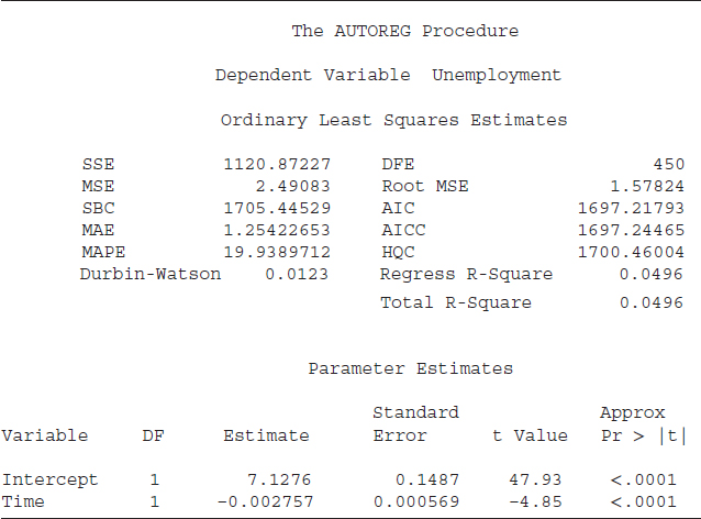
The Schwarz Bayesian criterion (SBC) = 1705.44529 and Akaike information criterion (AIC) = 1697.21793 are information criteria and are helpful tools to select a model among its competitors. The mean absolute error (MAE) = 1.25422652 and mean absolute percentage error (MAPE) = 19.9389712 are measures of errors. There are two R² statistics reported in Table 6.5, “Regress [Regression] R-Square” and “Total R-Square.” The regression R² is a measure of the fit of the structural part of the model after transforming for the autocorrelation and thereby is the R² for the transformed regression. The total R² is also a measure of how well the next value of a dependent variable can be predicted using the structural part of the equation (right-hand-side variables including the intercept) and the past value of the residuals (estimated error term). Furthermore, if there is no correction for autocorrelation, then the values of the total R² and regression R² would be identical, as in our case, where both total and regression R² are equal to 0.0496. Another important statistic shown in Table 6.5 is the Durbin-Watson statistic, which is equal to 0.0123. A Durbin-Watson statistic close to 2 is an indication of no autocorrelation and a value close to zero, as in present case, is a strong evidence of autocorrelation—not a good sign.

The last part of Table 6.5 reports statistics to measure the statistical significance of the right-hand-side variables (independent variable[s] along with an intercept). The column under the name “Variable,” shows the name of the intercept and independent variable, in this case “Time.” The “DF” represents degrees of freedom; “1” indicates 1 degree of freedom for each parameter. The next column, “Estimate,” shows the estimated coefficients for the intercept (7.1276) and for time (–0.002757). The next column exhibits the “Standard Error” of the estimated coefficient. This is a very important statistic for three reasons.

1. The standard error of a coefficient indicates the likely sampling variability of a coefficient and hence its reliability. A larger standard error relative to its coefficient value demonstrates higher variability and less reliability of the estimated coefficient.
2. The standard error is an important input to estimate a confidence interval for a coefficient. A larger standard error relative to its coefficient provides a wider confidence interval.
3. The coefficient relative to the standard error helps to determine the value of a t-statistic. An absolute t-value of 2 or more is an indication that the variable is more likely to be statistically useful to explain the variation in the dependent variable. In this case, both t-values, in absolute terms, are greater than 2 (47.93 for intercept and −4.85 for time), suggesting that both the intercept and time are statistically significant.

The last column, “Approx Pr > |t|,” represents the probability level of significance of a t-value. Basically, this column indicates at what level of significance we can reject (or fail to reject) the null hypothesis that a variable is statistically significant. The standard level of significance is 5 percent; an “Approx Pr > |t|” value of 0.05 or less will be an indication of statistical significance. The values for both t-values are smaller than 0.05 (both are 0.0001); hence the intercept and time are statistically meaningful to explain variation in the unemployment rate. The negative sign of the time coefficient (–0.002757) demonstrates that the unemployment rate may have a downward time trend. It is statistically significant, as the t-value is greater than 2, which shows that the time trend may be linear.

SAS code S6.12 estimates a nonlinear (quadratic) trend for the unemployment rate. The first and the last lines of the code are identical to code S6.11. The difference is in the middle line. We added Time_2, which is square of the time dummy variable, and included it in the regression analysis to capture any nonlinearity of the time trend.

The results based on code S6.12 are reported in Table 6.6. Both SBC (1576.49193) and AIC (1564.15088) are smaller for the nonlinear model compared to the linear model. The t-values for the “Time”, “Time_2,” and the intercept are greater than 2, and the probability for the t-values is also smaller than 0.05, implying that these coefficients are statistically significant at the 5 percent level of significance. The negative sign of the “Time” and positive sign of “Time_2” imply that the unemployment rate may contain a nonlinear, U-shaped time trend.

Both SBC and AIC are smaller for the nonlinear trend model compared to the linear trend model and thereby we prefer a nonlinear trend model to estimate the unemployment rate.

TABLE 6.6 SAS Output Based on the PROC AUTOREG: A Nonlinear Time Trend

SAS code S6.13A estimates a log-linear trend for the unemployment rate. The dependent variable is the log of the unemployment rate instead of its level.¹⁷ The results based on the log-linear trend model are displayed in Table 6.7A. Both SBC and AIC are smallest for the log-linear trend model compared to the previous two models. The t-value indicates that the Time variable is statistically significant.

Although the log-linear trend model has smaller SBC and AIC values compared to the linear and nonlinear trend models, the log-linear model used the log of the unemployment rate. The other two models are based on the level form of the unemployment rate. It may not be accurate to compare SBC and AIC among these three models because of different forms of the dependent variable. Because for the sake of comparison we need an identical dependent variable for all three models, which is the level form of the unemployment rate. Therefore, we run another model for the log-linear trend and that model uses the level form of the unemployment rate as a dependent variable and exponential form of the Time variable as a right-hand-side variable.

Because it is more flexible, we employ the PROC MODEL to estimate the exponential trend model for the unemployment rate. Unfortunately, we could not estimate the above regression through the PROC AUTOREG although it produces SBC and AIC values automatically which the PROC MODEL can't do. Both procedures thus have some advantages and some limitations.

The first line of the S6.13B code is similar to the S6.13A code; the only difference is that we are using the PROC MODEL instead of the PROC AUTOREG. The second line shows the regression equation which we are interested in estimating. That is, unemployment = a0 + exp (a1*Time) where unemployment is the dependent variable and a0 is a user-defined SAS name for the intercept. exp is a SAS keyword that instructs SAS to use the exponential form of the variable in the estimation process. a1 is the slope coefficient, and Time is time dummy variable. exp (a1*Time) implies that the exponential form of the Time variable is used in the regression analysis. The next line of the code starts with fit, which is a SAS keyword that instructs SAS to fit the model for unemployment. fiml stands for “Full Information Maximum Likelihood”; it is an estimation method.¹⁸ We employed FIML because it will estimate likelihood values, and that is an important input to calculate SBC and AIC.

Results based on the S6.13B are reported in Table 6.7B. Any time we employ the PROC MODEL, we obtain results similar to those displayed in that table.

The first row of Table 6.7B states that the PROC MODEL is employed, and second row indicates the FIML is the estimation method. The regression equation is fitted for the unemployment rate. “DF Model” stands for the model's degree of freedom; it is 2 because there are only two parameters, ao (the intercept) and a1 (the slope coefficient). “DF Error” is the degrees of freedom for the error, and it is 450. It is equal to total number of observations (which are 452) minus the DF model (which is 2). The next columns show SSE, MSE, and R² statistics. PROC MODEL also provides an adjusted R² (Adj R-Sq), which equals 0.0824. The next part of the table provides estimated coefficients and their measures of statistical significance. The a1 is attached to a t-value of −1.50, and probability for that t-value is 0.1349, which implies that the Time variable is statistically insignificant at the 5 percent level of statistical significance.

TABLE 6.7A SAS Output Based on the PROC AUTOREG: A Log-Linear Time Trend

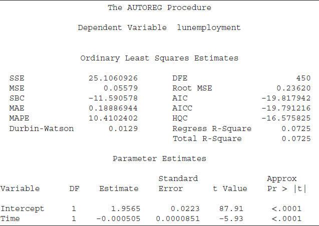
TABLE 6.7B SAS Output Based on the PROC MODEL: A Log-Linear Time Trend

The last section of Table 6.7B shows the number of observations used in the regression analysis (452) and the log likelihood, which is −838.1754. PROC MODEL does not provide SBC and AIC, which are important inputs to select the appropriate trend model for the unemployment rate. However, SBC and AIC can be calculated by hand using these formulas:

where

ln =	Natural logarithm
L =	value of the likelihood function (−838.1754)
N =	number of observations (452)
k =	number of estimated coefficients including the intercept (2)

The estimated value of the SBC is 1681.66 and for AIC is 1680.35.

Table 6.8 summarizes the SBC and AIC value for all three of the trend models we have discussed. The nonlinear model has the smallest SBC value as well as the smallest AIC value. We thus conclude that for the U.S. employment rate, a nonlinear trend model would be the most appropriate model.

Identifying Cyclical Behavior in a Time Series

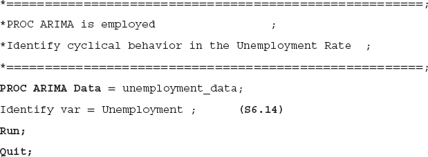
Identifying cyclical behavior in a time series is vital for decision makers. A series that contains cyclical behavior is easier to analyze during a particular phase of a business cycle. We employ PROC ARIMA to identify cyclical behavior and use the U.S. unemployment rate as a case study.

The first line of code S6.14 shows that PROC ARIMA is employed and the unemployment_rate dataset is used in the analysis. In the second line of the code, Identify var = Unemployment, Identify and var are SAS keywords that instruct SAS to estimate autocorrelations and partial autocorrelation functions for the variable, in this case for unemployment rate.¹⁹ Basically, the second line of the code asks SAS to provide autocorrelations and partial autocorrelation functions, which are important ingredients to determine whether a time series contains cyclical behavior.

TABLE 6.8 The SIC/AIC of All Three Models

The results based on the S6.14 code are displayed in Tables 6.9A to C. The first part of Table 6.9A shows basic statistics for the unemployment rate. That is, the mean and standard deviation of the unemployment rate are 6.5030 and 1.6153, respectively. A total of 452 observations are used in the analysis.

TABLE 6.9A SAS Output Based on the PROC ARIMA

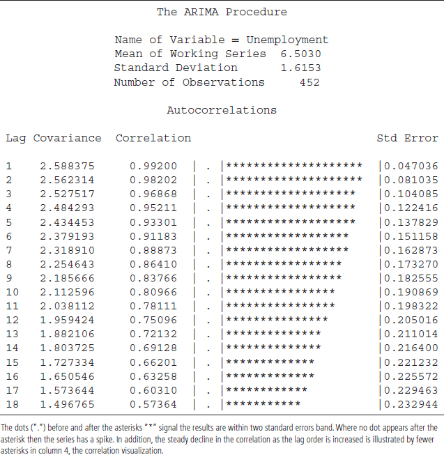
The second part of Table 6.9A shows a plot for the autocorrelation functions (ACFs). The ACFs plot indicates that the autocorrelations are larger relative to two standard-error bands (dotted line) at least for several lags. The ACFs also display a slow decay in the autocorrelations compared to the two standard-error bands. These are the first two conditions for identifying cyclical behavior. The ACFs also show that the unemployment rate contains cyclical behavior.²⁰ In Table 6.9B, the partial autocorrelations functions (PACFs) plot reveals a large spike at the first lag, confirming the ACFs' findings. Essentially, both ACFs and PACFs are providing strong evidence of cyclical behavior in the unemployment rate.

Table 6.9C provides results based on the autocorrelation test for various lag orders. The null hypothesis of the test is no autocorrelation and the alternative hypothesis is that autocorrelation is present. The first column of the table shows the lag order, how many lags of unemployment rate are used to estimate an autocorrelation. The second column provides “Chi-Square” test values and the third column indicates “DF,” or degrees of freedom. The fourth column, “Pr > ChiSq” provides probabilities attached to the Chi-square test values. Since the probability values are significantly smaller than 0.05, we reject the null hypothesis of no autocorrelation at 5 percent level of significance, therefore concluding again that autocorrelation is present.

TABLE 6.9B SAS Output Based on PROC ARIMA

TABLE 6.9C SAS Output Based on PROC ARIMA

Since the presence of autocorrelation indicates that the unemployment rate shows a persistent pattern, periods of relatively higher unemployment rates may be associated with other periods of relative higher unemployment rates. That is, during recessions and the early phases of a recovery, unemployment rates may stay at an elevated level for a while. A good example of this is the U.S. unemployment rate during the 2008 to 2012 period, when unemployment stayed elevated at around 9 percent plus. The last part of Table 6.9C provides autocorrelations functions values, which are identical to those provided in Table 6.9A.

Modeling Cyclical Behavior: Identify AR(p) and MA(q)

The ACFs, PACFs, and autocorrelation test findings provide strong evidence of cyclical behavior in the unemployment rate. The next step would be to model that cyclical behavior to predict the behavior of the unemployment rate. The modeling of cyclical behavior requires identification of autoregressive (AR) and moving average (MA) orders, in other words an ARMA (p, q).²¹ Most time series data involve a non-stationary characteristic, so we need to identify the order of integration, also called I(d), to determine whether the series is nonstationary or not. We combine the process to identify the orders of AR (p), MA (q) and I(d), known as ARIMA, autoregressive integrated moving average.²²

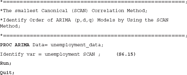
SAS software provides a user-friendly method to tentatively identify the order of candidate ARMA or ARIMA models, known as the SCAN method for the smallest canonical correlation approach.²³

The SAS code in S6.15 identifies the orders of AR(p), MA(q) and I(d), using the U.S. unemployment rate as a case study. In the second line of the code, we added the SAS keyword SCAN, which instructs SAS to identify tentative ARMA/ARIMA order for unemployment rate using the SCAN method. We ended the S6.15 code with Run and Quit.²⁴

Tables 6.10 and 6.11 are based on SAS code S6.15. The first part of Table 6.10 provides squared canonical correlation estimates; the second part shows the SCAN Chi-square probability value of the test. We highlighted the MA (1); and AR (2), and the corresponding value, 0.3708. The value 0.3708 is the first one that is greater than 0.05 and implies that, at a 5 percent level of significance, we failed to reject the hypothesis of no correlation. This indicates that the unemployment may be modeled using one of the following candidate models: ARMA(2,1), ARIMA(1,1,1) or ARIMA(0,2,1). Each of these three models can be estimated using PROC ARIMA and the AIC and/or SBC statistics can be compared to select the best-fitting model. The SCAN method summarizes the results and provides a tentative order of ARIMA in Table 6.11.

TABLE 6.10 SAS Output Based on PROC ARIMA: The SCAN Method

TABLE 6.11 Tentative Order Selection Tests

The PROC ARIMA and SCAN methods are powerful tools to identify the model for the cyclical behavior of a time series. By using these tools, we can conclude that the U.S. unemployment rate contains cyclical behavior. Furthermore, the SCAN method suggests a p + d order equal to 2 and MA (1). That is, in the modeling process of the unemployment rate, it would better to use lag-1 of the unemployment rate as right-hand-side variables and also lag-1 of the error term (as MA(1)) as a right-hand-side variable in the test equation.²⁵

SUMMARY

This chapter provides useful tips for users to get started in SAS. By utilizing several econometric techniques, an analyst can characterize different time series through SAS. We wish to stress that the first step of an applied time series analysis is to understand the behavior of a time series, which helps during modeling and forecasting. An analyst should plot a variable over time for visual inspection (i.e., to determine whether the series has a trend, cyclical behavior, etc.). In a next step, calculation of the mean, standard deviation, and stability ratio over different business cycles will help the analyst to understand the series behavior over time.

Formal trend estimation of a time series is also essential, as it helps analysts to determine whether a series has an upward or downward trend over time. By characterizing the cyclical behavior of a series, an analyst can learn the series' behavior over different phases of a business cycle.