
19
RISK, UNCERTAINTY, AND THE COST OF CAPITAL
CHAPTER INTRODUCTION
Risk and uncertainty impact all projections about future performance that support everything from forecasts and plans to investment decisions and valuations. We will deal with uncertainty in this chapter in the form of discounting future cash flows. Risk and uncertainty are addressed, in part, in two fundamental financial principles: the time value of money and the cost of capital. Additional mechanisms to understand and deal with risk and uncertainty are addressed in Chapters 20 and 21 covering capital investment decisions.
THE TIME VALUE OF MONEY
The time value of money (TVOM) is an important financial concept. Essentially, the TVOM recognizes that a dollar today is worth more than an expectation of receiving a dollar in the future. Several factors contribute to this:
- Inflation reduces the purchasing power in the future.
- Uncertainty reduces the value of future cash or income payments (you may never get paid in full).
- If you hold or invest a dollar, there is an “opportunity cost” (i.e. you are forgoing other opportunities to use that dollar). If you leave your savings in a passbook savings account with very modest interest rates, you have passed on an opportunity to invest in a stock or bond with potentially higher returns. If a company invests in a project, it is passing on the opportunity of investing the capital in another project or financial security (or returning it to shareholders).
We will review the key aspects of TVOM before proceeding to the cost of capital.
Compounding
Compounding is used to estimate the future value of a present sum. This enables us to estimate the future value of an investment, as in compound interest or compound growth rates.
Simple Compounding Illustration
Simple compounding is determining the future value (FV) of a present value (PV) or sum growing at an interest rate (i). The formula for determining the future value of a single cash flow for a single year is:

For multiyear compounding, that is, to determine the future value (FVn) of a sum growing at an interest rate (i) for multiple years (n), the formula is:

This growth in value or compounding is illustrated in Figure 19.1. Note an important feature of compounding: the interest earned in prior periods earns interest!

FIGURE 19.1 Compounding Illustration
Applications of compounding include:
- Calculating how much a $5,000 savings balance will grow to in 10 years.
- Estimating sales with a compound annual growth rate (CAGR).
Future Value of an Annuity
An annuity is a stream of equal cash flows that occur at regular intervals over time. Examples of annuities include determining the future value of a regular savings plan, such as contributions to a 401(k) or IRA. To compute the future value of an annuity (FVAn), with periodic payments (PMT) for (n) years, at a periodic interest rate (i), we use the following formula:

For example, what is the value in year 5 of annual contributions to an investment earning 10% per annum?

Figure 19.2 details the growth of each contribution and provides important insight into the TVOM. The initial $1,000 contribution grows to $1,464 over five years, while subsequent contributions have shorter periods to compound.
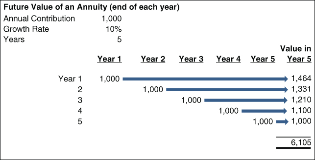
FIGURE 19.2 Future Value of Annuity Illustration
Application:
How much will my annual IRA contribution be worth in 20 years?
Discounting
Discounting is the methodology we employ to estimate the present value of a future sum or payment. Discounting is a key tool used in business and investment valuation and evaluating capital investments.
Discounting a Future Payment
Let us assume that we will get a $100,000 payment (FV) in four years (n) from today. Based on the risk and opportunity costs, we have determined that a 4% interest rate (i) is appropriate. What is the value of this future payment today (PV0), given this risk and opportunity cost? Figure 19.3 shows that the future payment must be discounted by 4% per year to arrive at the present value.

FIGURE 19.3 Discounting Illustration
The formula for computing the present value (PV0) of a future sum (FVn) is:

Application:
How much money do I need to invest today for n years to pay for my kids' college educations?
Discounting Future Cash Flows
In many business decisions, the future cash flows will be realized in several future periods. The cash flow for each of the periods will have to be estimated and then discounted to its present value. We'll start with a simple example, determining the present value of a bond (see Figure 19.4).

FIGURE 19.4 Bond Valuation Illustration
Bond Pricing Illustration:
How much should you pay for a $10,000 bond, maturing in two years, with a coupon rate of 7%, paid annually, if the current rate on comparable bonds is 10%?
The Value of an Annuity in Perpetuity
An annuity in perpetuity is a fixed payment every year, forever! In practice these rarely exist, but they provide a basis for valuing long‐term payment streams such as the value of annual payments to lottery winners and the terminal (or post‐horizon) value in business valuations (covered in Chapter 22).
Example:
What is the PVt on a $100,000 annuity (PMT) in perpetuity if the discount rate is 10% (i)? The present value of an annuity in perpetuity is computed as follows:

Present Value of a Growing Annuity in Perpetuity
A growing annuity in perpetuity provides a periodic cash flow that is expected to grow at a constant rate (g) forever. Examples include terminal values in valuation and in valuing stocks using the dividend method.

where PMTt + 1 = PMT next year.
Example:
What is the PV of a $100,000 annuity growing at 5% per year in perpetuity if the discount rate is 10%?

Note the significant difference from the value computed for the present value of an annuity in perpetuity ($1,000,000). This illustrates the importance of growth as a driver of value.
Present Value of Uneven Cash Flows
Frequently, the application of TVOM involves uneven cash flows over a number of years. This occurs in most real‐world business problems such as valuing businesses and acquisitions and capital investment decisions.
Uneven Cash Flows Illustration:
What is the present value (PV) of a project that requires a $1 million investment now, will generate cash flows of 0 in year 1, $50,000 in years 2 and 3, and $100,000 in year 4, and has an estimated terminal value in year 5 of $1.4 million? Assume a discount rate of 10%. Will the investment in this project create value for the firm? See Table 19.1.
TABLE 19.1 Uneven Cash Flows Illustration
| Year | 0 | 1 | 2 | 3 | 4 | 5 |
| Cash Flow | (1,000,000) | – | 50,000 | 50,000 | 100,000 | 1,400,000 |
| Present Value Factor (PVF) | 1.000 | 0.909 | 0.826 | 0.751 | 0.683 | 0.621 |
| Present Value (PV) | (1,000,000) | – | 41,322 | 37,566 | 68,301 | 869,290 |
| NPV (Sum of Present Value) | 16,479 | |||||
| Discount Rate | 10% |
The construction of cash flow timeline by year is the critical first step. Next, we will compute the present value factor (PVF) for each year and multiply the cash flow for each year by the respective PVF. The sum of the PVs of cash flows for each year is known as the net present value (NPV).
As we will fully explore in Chapter 20, Capital Investment Decisions: Introduction and Key Concepts, this project has a positive NPV, indicating that the project will create value and should be approved and implemented.
Discounting uneven cash flows will be utilized throughout Part Five, Valuation and Capital Investment Decisions.
THE COST OF CAPITAL
Introduction
The cost of capital is a significant determinant of shareholder value. It is the rate used by investors to discount future cash flows, as shown in Figure 19.5. For investors that value companies using multiples of earnings or sales, it is one of the implicit assumptions made in selecting the multiple to use. Value is inversely related to the cost of capital. As the cost of capital declines, the value of the firm will increase, and vice versa.

FIGURE 19.5 Discounted Cash Flow (DCF)
Cost of capital can have a significant impact on the value of a firm. Figure 19.6 plots the relationship between cost of capital and enterprise value for Roberts Manufacturing Company based on the DCF model used in Chapter 22.

FIGURE 19.6 Sensitivity of Value to Cost of Capital 
A fundamental aspect underlying the cost of capital is the relationship between risk and return. We all recognize that a riskier investment must have a higher potential return than a safer one, as otherwise we would simply invest in the safer investment. For example, few sensible people would invest in a start‐up company that, if successful, was expected to return a rate close to the risk‐free rate on US Treasury bonds. Most would invest in the much safer investment providing the same return. We all would expect a risk premium for the higher‐risk start‐up investment. This risk‐return trade‐off is pictured in Figure 19.7.

FIGURE 19.7 Risk and Return
Cost of Capital Drivers
The cost of capital for a firm is driven by several factors as illustrated in Figure 19.8, including interest rates, financial and operating leverage, volatility, and risk.

FIGURE 19.8 Cost of Capital Drivers
Market Interest Rates
The starting point in determining the cost of capital is typically the risk‐free rate of return. Investors have the opportunity to invest in an essentially risk‐free investment, US Treasury notes. This rate will form the baseline for setting required rates of return for alternative investments with progressively higher risks.
Financial Leverage
Another significant driver of the cost of capital for a firm is the mix of capital used to run the business. Typically, the cost of debt is lower than the cost of equity, as interest rates are generally well below expected rates of return on equity investments. In addition, the cost of debt is reduced by the related tax savings, since interest expense is a deduction in computing taxable income in most cases.
Operating Leverage
Operating leverage refers to the composition of costs and expenses for a company and was covered in detail in Chapter 3. A firm that has most of its costs fixed in the short term is said to have a high degree of operating leverage. A change in sales levels will have a dramatic effect on profits for this firm, since most of its costs are fixed. By contrast, a company with lower operating leverage has a greater portion of its cost structure as variable. That is, if sales decline, the variable costs will also be reduced. The firm with high operating leverage will experience greater fluctuations in profits and cash flows for a given change in sales, leading to a higher level of volatility and perceived risk.
Volatility and Variability
Companies that have unpredictable or inconsistent business results typically are valued at a discount to companies with predictable and consistent operating performance. Investors using multiples to value a highly volatile business will use a lower multiple of sales or earnings. Investors that employ discounted cash flows will use a higher weighted average cost of capital (WACC), used to discount future projected cash flows.
Perceived Risk
Investors will demand returns commensurate with the risk level they perceive in a business. Examples of additional factors leading to higher perceived risk:
- Geopolitical factors, for example developing countries or unstable regions
- Currency exposure
- Competitive pressure
- Technological obsolescence
- Management departures
Estimating the Cost of Capital
The most common method used to estimate the cost of capital is the weighted average cost of capital (WACC) method. The WACC methodology computes a blended or weighted cost of capital, considering that capital is often supplied to the firm in various forms. The most common are equity, provided by shareholders, and debt, provided by bondholders. In addition, there are many other forms that combine elements of both debt and equity. Examples of these hybrid securities include preferred stock and convertible bonds. It is important to emphasize that the cost of capital represents an estimate or approximation. Recognizing this, we should test the inputs to the WACC formula and use sensitivity analysis to understand the impact of these assumptions on the valuation of a company.
WACC Computation
Following are the steps to compute the WACC:
- Estimate the cost of equity.
- Estimate the cost of debt.
- Weight the cost of equity and debt to compute the WACC.
The information in Table 19.2 will be used to illustrate the WACC computation.
TABLE 19.2 WACC Illustration Inputs
| Market Information | |
| Current Risk‐Free Rate on US Treasury Notes | 4.0% |
| Historical Market Premium for Stocks (vs. Risk‐Free) | 5.5% |
| Company Information: | |
| Market Value of Equity ($ millions) | 90.0 |
| Beta of Company Stock (Measure of Volatility) | 1.09 |
| Market Value of Debt ($ millions) | 10.0 |
| Interest Rate (Yield to Maturity*) YTM | 6.0% |
| Tax Rate | 40% |
*Yield to maturity is used in WACC computation, not coupon rate.
Step 1: Estimate the Cost of Equity
The cost of equity represents the estimated return expected by shareholders and potential shareholders. Three components are considered: the risk‐free rate, the premium expected for equity investments (market premium), and risk attributable to the specific company (beta). The cost of equity for this firm would be computed as follows:

Step 2: Estimate the Cost of Debt
Since interest expense is generally tax deductible, the cost of debt is reduced by the tax savings and is computed as follows:

Step 3: Weight the Cost of Equity and Debt to Compute WACC
Table 19.3 shows the WACC computation.
TABLE 19.3 WACC Computation ![]()
| Market | Market | |||
| Cost | Value | Value % | Weighting | |
| Debt | 3.6% | 10.0 | 10% | 0.36% |
| Equity | 10.0% | 90.0 | 90% | 9.00% |
| Total/WACC | 100.0 | 100% | 9.36% |
Figure 19.9 provides a visual summary of how these elements come together in the WACC computation. Investors that invest in equity securities expect a premium over returns obtainable from risk‐free securities (US Treasury notes). This market premium results in an expected return for the market (e.g. S&P 500), in the illustration, just above 10%. The cost of capital for a particular security is then computed by adding a premium for the risk of investing in an individual security. The cost of equity is then blended with the after‐tax cost of debt to estimate the weighted average cost of capital.

FIGURE 19.9 WACC Visual Summary
Since the cost of debt is typically lower than the cost of equity, it is easy to conclude that some blend of debt and equity would result in the lowest cost of capital. The combination of debt and equity that results in the lowest cost of capital is called the optimal capital structure. This concept is illustrated in Figure 19.10. A firm with no debt will have a WACC equal to the cost of equity. As the firm adds debt to the mix, the WACC will be reduced to a point. However, at some point the increased risk associated with high borrowings will increase the required interest rates and will also increase the required cost of equity. The combined effects will increase the WACC above the minimum level projected at the optimum capital structure.

FIGURE 19.10 Optimal Cost of Capital and Capital Structure
Most firms do not operate at or near the optimal capital structure. There are several reasons for this. First, some managers do not fully accept the concept of discounted cash flow/cost of capital or WACC. Others are very conservative and are opposed to the risk introduced by using or increasing debt. Even managers that accept the basic concept choose not to add leverage, or will add reasonable levels of debt that leave them far short of the theoretical optimum capital structure. Typically, companies will set a target capital structure, expressed as a ratio of debt to total capital, for example 30% to 40%. Figure 19.11 captures some of the factors that influence decision makers in setting a target capital structure. Tolerance for risk, capital requirements, and growth rates are a few examples. Firms will then often deviate from this target capital structure. For example, they may choose to exceed the target range to finance a strategic opportunity such as an acquisition. Typically, the corporation would plan to return to the target range within a couple of years or reset the range to a higher level.

FIGURE 19.11 Capital Structure and Financial Policy
Key Ways Managers Can Reduce the Cost of Capital
Some of the factors that determine cost of capital are out of the firm's control. For example, market interest rates are the foundation for estimating cost of capital. Unless they have influence over the general economy, inflation, or the chairman of the Federal Reserve Bank, there is little managers can do about interest rates. Here are some specific actions managers can take to reduce the cost of capital:
- First, managers can reduce surprises and volatility, which will result in a lower beta and cost of capital and therefore higher valuation. Managers should strive to improve the predictability and consistency of business performance for several reasons. In addition to reducing surprises and volatility that affect the cost of capital, improvements in this area will result in lower working capital requirements and operating costs.
- Second, managers can consider using a reasonable level of debt in the capital structure. Utilizing a sensible level of debt provides leverage to equity investors and reduces the cost of capital. The level of debt should be lower than theoretical borrowing capacity, to provide for a cushion to service this debt during a business downturn or unforeseen future challenges.
- Third, managers can improve communications with investors. To the extent that investors have a full understanding of the business performance and potential, they will likely have a better perspective on the business. This better understanding and perspective will result in reducing potential overreactions to expected variations in business performance.
PERFORMANCE MEASURES
A number of measures can be tracked to provide insight into the firm's WACC and identify potential opportunities to reduce the cost of capital.
Financial Leverage: Debt to Total Capital
In Chapter 2, we reviewed key financial ratios that measure financial leverage and capital structure. The mix of debt and equity in the capital structure is an important variable in the cost of capital and valuation. For evaluating financial leverage, the measure is usually computed using book values:

Stock Volatility/Beta
For a public company, the volatility of the company's stock price is an important indicator of the level of risk perceived by investors. Investors attempt to estimate the risk inherent in future performance and cash flows by looking at historical measures of stock volatility or beta. Beta compares the change in the firm's stock price to the change in a broad market measure. Beta, which measures the correlation of an individual stock to the S&P 500, is available in many financial reporting services. Services use different time horizons to calculate beta and stock volatility, often going back several years. Since we want to track beta or stock volatility to use in estimating a cost of capital for future performance, we must ensure that the historical measure is indicative of future performance. Care should be exercised in circumstances where significant changes have recently occurred, or are anticipated, in the company's market, strategic direction, or competitive environment. In these cases, managers and investors may focus on recent history or expected future stock price volatility or beta as a better indicator of current investor confidence and perceived risk.
Operating Leverage
In Chapter 3 we concluded that the mix of variable and fixed cost components has a significant impact on the earnings and cash flow of a firm as sales levels vary. Where sales volatility is likely, for example in cyclical businesses, managers should closely monitor and evaluate the cost structure of the company. Fixed cost levels or breakeven sales levels should be measured and evaluated periodically.

FIGURE 19.12 Cost of Capital Dashboard
Actual versus Projected Performance
Preparing business forecasts is an important activity for most companies. These forecasts will be the basis for making important decisions and in investor communications. For many firms, future estimates of revenue are typically the most important and difficult operating variables to forecast. In Part Three: Business projections and Plans, we presented a number of tools to monitor and evaluate the accuracy and effectiveness of forecasts. Forecast variances should also be reviewed in the context of the firm's cost of capital, since the predictability and consistency of operating performance will affect stock volatility.
Illustrative Dashboard: Cost of Capital
A dashboard for the cost of capital should be utilized, incorporating key performance indicators appropriate to the specific issues and priorities for each company. An illustrative cost of capital dashboard is presented in Figure 19.12.
SUMMARY
The time value of money is a core financial concept. Simply stated, a dollar promised in the future is worth less today. The value today must recognize risk and the opportunity cost of not having that dollar today to invest in other alternatives.
The cost of capital for a firm is a significant value driver. Cost of capital is inversely related to the firm's value. Managers should be aware of the sensitivity of the company's valuation to the cost of capital. Management can reduce the cost of capital, thereby increasing value, by reducing risk and volatility and by using an appropriate mix of debt and equity. Key factors impacting the firm's cost of capital should be identified and measured.