With roscore running, start rqt_rviz with (note that rviz is still valid in ROS hydro):

$ rosrun rqt_rviz rqt_rviz

We will see the graphical interface of the following screenshot, which has a simple layout:

On the left-hand side, we have the Displays panel, in which we have a tree list of the different elements in the world, which appears in the middle. In this case, we have certain elements already loaded. Indeed, this layout is saved in the config/example9.rviz file, which can be loaded in the File | Open Config menu.

Below the Displays area, we have the Add button that allows adding more elements by topic or type. Also note that there are global options, which are basically a tool to set the fixed frame in the world, with respect to which the others might move. Then, we have Axes and a Grid as a reference for the rest of the elements. In this case, for the example9 node, we are going to see Marker and PointCloud2.

Finally, on the status bar, we have information regarding the time, and on the right-hand side, there are menus. The Tools properties allows us to configure certain plugin parameters, such as, the 2D Nav Goal and 2D Pose Estimate topic names. The Views menu gives different view types, where Orbit and TopDownOrtho are generally enough; one for a 3D view and the other for a 2D top view. Another menu shows elements selected on the environment. At the top, we also have a menu bar with the current operation mode (Interact, Move, Measure, and so on.) and certain plugins.

Now we are going to run the example9 node using the following screenshot:

$ roslaunch chapter3_tutorials example9.launch

In rqt_rviz, we are going to set frame_id of the marker, which is frame_marker, in the fixed frame. We will see a red cubic marker moving, as shown in the following screenshot:

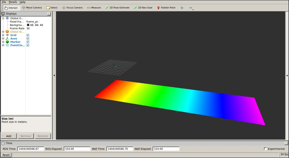
Similarly, if we set the fixed frame to frame_pc, we will see a point cloud that represents a plane of 200 x 100 points, as shown in the following screenshot:

The list of supported built-in types in rqt_viz includes Camera and Image, which are shown in a window—similar to image_view. In the case of Camera, its calibration is used, and in the case of stereo images, they allow us to overlay the point cloud. We can also see the LaserScan data from range lasers, Range cone values from IR/sonar sensors, or PointCloud2 from 3D sensors, such as the Kinect sensor.

For the navigation stack, which we will cover the in next chapters, we have several data types, such as Odometry (which plots the robot odometry poses), Path (which draws the path plan followed by the robot), Pose objects, PoseArray for particle clouds with the robot pose estimate, the Occupancy Grid Map (OGM) as a Map, and costmaps (which are of the Map type in ROS hydro and were GridCell before).

Among other types, it is also worth mentioning the RobotModel, which shows the CAD model of all the robot parts, taking the transformation among the frames of each element into account. Indeed, tf elements can also be drawn, which is very useful to debug the frames in the system; we will see an example in the next section. In RobotModel, we also have the links that belong to the robot URDF description with the option to draw a trail showing how they move over time.

Basic elements can also be represented, such as a Polygon for the robot footprint; several kind of Markers, which support basic geometric elements, such as cubes, spheres, lines, and so on; and even InteractiveMarker objects, which allow the user to set a pose (position and orientation) on the 3D world. Run the example8 node to see an example of a simple interactive marker:

$ roslaunch chapter3_tutorials example10.launch

You will see a marker that you can move in the interactive mode of rqt_rviz. Its pose can be used to modify the pose of another element in the system, such as the joint of a robot:

All topics must have a frame if they are publishing data from a particular sensor that has a physical location in the real world. For example, a laser is located in a position with respect to the base link of the robot (usually at the middle of the traction wheels in wheeled robots). If we use the laser scans to detect obstacles in the environment or to build a map, we must use the transformation the laser and the base link. In ROS, stamped messages have frame_id, apart from the timestamp (which is also extremely important to put or synchronize different messages). A frame_id gives a name to the frame it belongs to.

However, the frames themselves are meaningless. We need the transformation among them. Actually, we have the tf frame, which usually has the base_link frame as its root (or map if the navigation stack is running). Then, in rqt_rviz, we can see how this and other frames move with respect to each other.

To illustrate how to visualize frame transformations, we are going to use the turtlesim example. Run the following command to start the demonstration:

$ roslaunch turtle_tf turtle_tf_demo.launch

This is a very basic example with the purpose of illustrating the tf visualization in rqt_rviz; note that, for the different possibilities offered by the tf API, you should see later chapters of this book. For now, it is enough to know that it allows us to make computations in one frame and then transform them to another, including time delays. It is also important to know that tf is published at a certain frequency in the system, so it is like a subsystem where we can traverse the tf tree to obtain the transformation between any frames in it; we can do it in any node of our system just by consulting tf.

If you receive an error, it is probably because the listener died on the launch startup because another node that was required was still not ready, so please run the following command on another terminal to start it again:

$ rosrun turtle_tf turtle_tf_listener

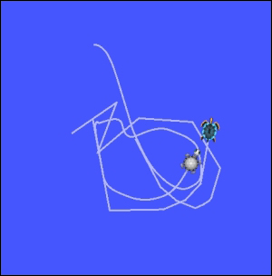
Now you should see a window with two turtles, where one follows the other. You can control one of the turtles with the arrow keys as long as you have the focus on the terminal where you run the launch file. The following screenshot shows how one turtle has been following the other after moving the one we control with the keyboard for some time:

Each turtle has its own frame, so we can see it in rqt_rviz:

$ rosrun rqt_rviz rqt_rviz

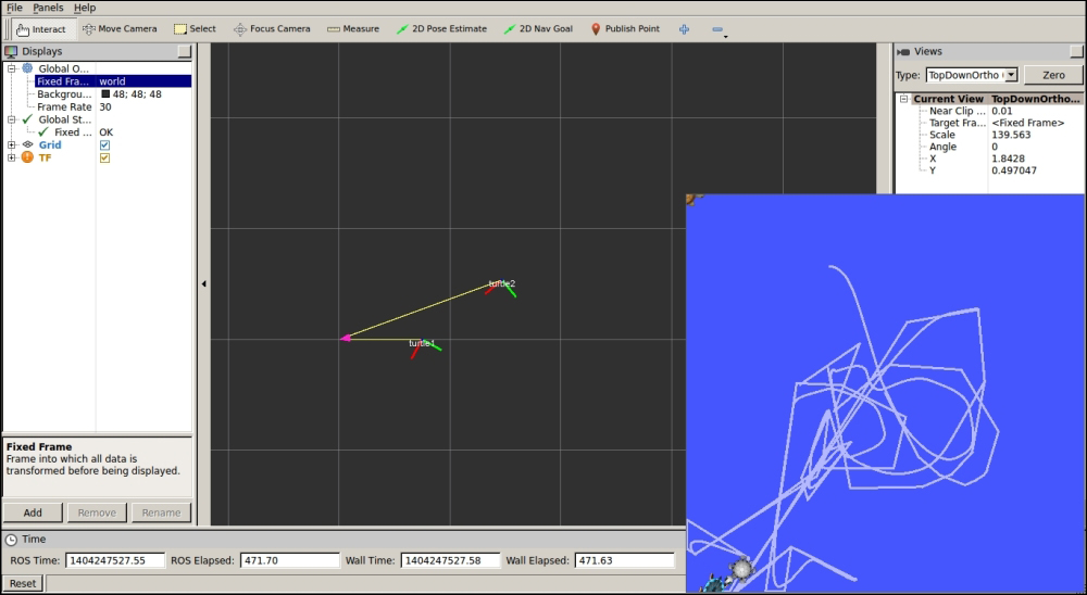
Now, instead of viewing the turtlesim window, we are going to see how the turtles' frames move in rqt_rviz as we move our turtle with the arrow keys. We have to set the fixed frame to /world and then add the tf tree to the left-hand side area. We will see that we have the /turtle1 and /turtle2 frames, both as children of the root /world frame. In the world representation, the frames are shown as axes, and the parent-child links are shown with a yellow arrow that has a pink end. Also set the view type to TopDownOrtho, so it is easier to see how the frames move because they only move on the 2D ground plane. You might also find it useful to translate the world center, which is done with the mouse with the Shift key pressed.

In the next screenshot, you can see how the two turtle frames are shown with respect to the /world frame. You can change the fixed frame to experiment with this example and tf. Note that config/example_tf.rviz is provided to give the basic layout for this example: