
2.5 SUMMARY
The data available from the Phase Zero program comprise calibrated clutter files covering all of the clutter within the field-of-view from 106 different sites. Extensive analyses of these data lead to an understanding of a basic unifying mechanism underlying what appears at first consideration to be extreme variability and little predictability in low-angle clutter spatial amplitude distributions. This understanding is based on the fact that, at the very low angles of illumination of surface radar, ground clutter largely consists of backscatter from a sea of discrete clutter sources. That is, a wave is skimming over the landscape at grazing incidence, and backscatter is being measured from all the vertical sources that rise up from the landscape. Such discrete f0revertical sources may be natural or cultural and comprise such things as: roads and field boundaries (or, more specifically, the vertical objects clustered along them); buildings (usually in clusters or complexes, for example, at farmsteads and industrial facilities, along road and rail lines, in towns and villages); trees (isolated trees, or tree lines, as at the edge of forest cover, or as shelter belts, or along river valleys); or even high points in terrain or breaks in terrain slope (for example, that occur in hummocky, hilly, or mountainous regions, or at edges of river valleys). All such clutter sources are spatially localized and thus discrete.
Numerous low reflectivity or shadowed cells occur between cells containing discrete clutter sources, even though the overall region from which the clutter amplitude distribution is being formed is under general illumination by the radar. In other words, at very low angles, small rises in terrain throw long ground shadows and even unshadowed terrain surfaces near grazing incidence backscatter very weakly. The combination of many shadowed or low-reflectivity weak cells together with many discrete-dominated strong cells causes extreme spread in the resultant low-angle amplitude distributions in which individual samples of clutter strength vary over orders of magnitude. As illumination angle increases, the low reflectivity areas between discrete vertical features become more strongly illuminated, resulting in less shadowing and a rapid decrease in the spread of the distributions. The upper tails of the clutter distributions, however, and the mean strengths that are largely determined by the upper tails are still primarily caused by discrete sources and increase more slowly with increasing illumination angle.
Therefore, as a unifying mechanism, depression angle (i.e., the angle below the horizontal at which a clutter patch is observed at the radar) as it affects shadowing on a sea of discretes is the most important parameter at work in low-angle ground clutter data, even at the very low angles (typically, < 1°) and small (typically fractional) variations in angle that occur in surface-sited radar. This basic parametric dependence in ground clutter spatial amplitude distributions is such that strengths increase and spreads decrease as depression angle rises and percent shadowing falls. Attempts to refine this basic dependency through use of grazing angle (i.e., the angle between the tangent to the local terrain surface at the terrain point and the direction of illumination) have met with little additional success (but see Appendix 4.D). Reasons contributing to this lack of success include the extreme complexity that exists in terrain surfaces, the lack of detailed information defining these surfaces such that slopes (i.e., rates of change of elevation) are accurate, and difficulties in formulating a quantitative definition of terrain slope uniformly applicable across the various physical scales (centimeters to kilometers) at which slopes exist in landscape. Over and above such considerations of scale and accuracy in terrain elevation data is the fact that the backscatter is frequently dominated by vertical elements of land cover irrespective of the underlying terrain slope.
Chapter 2 presents preliminary low-angle X-band ground clutter modeling information for clutter amplitude statistics within a construct that requires relatively detailed specification of depression angle, but that requires specification of terrain type minimally as one of just three types—rural/low-relief, rural/high-relief, or urban. Terrain slope enters the model explicitly through the two categories of relief. This basic information is refined by providing additional results for more specific terrain types—e.g., farmland, forest, wetland, mountains. The modeling information is presented largely in terms of Weibull coefficients. The low-angle heterogeneous regime of widespread spiky Weibull statistics applicable to surface radar gradually transitions with increasing depression angle to the high-angle, more homogeneous regime of Rayleigh statistics applicable to airborne radar.
Chapter 2 emphasizes the importance of spatially localized or discrete sources in low-angle clutter statistics. The dominant role of discrete sources is not, in itself, a new idea in the clutter literature. Clutter models, however, have traditionally been developed, first, on a basis of area-extensive scattering from the statistically rough surface itself, as opposed to localized scattering from just the high points of that surface or high objects on it. One of the more valuable results of the Phase Zero clutter program is that low-angle clutter is now imagined as arising, first, from a sea of discrete vertical features or edges, separated by microshadow, and distributed over complex surfaces. The role of illumination angle in this construct is more as depression angle influences clutter strength through its effect on shadowing statistics between discrete features of vertical discontinuity, and less in the influence of grazing angle on area-extensive backscatter from tilted, statistically rough, terrain facets, although both sorts of illumination angle effects are at work in the actual phenomenon. Chapter 2 provides information on how clutter amplitude distributions vary with percent tree cover, which indicates that the dominant sources causing much of the wide spread typically observed in these distributions in open terrain are trees.
The problem of making radar ground clutter understandable and predictable is as much one of statistics as of physics. Given enough time and effort, the backscattering processes within and contributions from any particular clutter patch can be understood, but the heterogeneity of terrain often prevents useful generalization of such particular results. The ambiguous state of the historical clutter literature fundamentally reflects this problem. Hence the approach taken in this book is empirical, involving measurements from many patches and across many sites. This approach bounds the problem of clutter strengths for various terrain types by presenting generalized data with considerable averaging across sites and patches and not data specific to some particular clutter scene that is nonrepresentative of other scenes.
Appendix 2.A PHASE ZERO RADAR
2.A.1 PHASE ZERO RADAR
The Phase Zero clutter measurement radar was based on an X-band commercial marine navigation radar—the Raytheon Mariners Pathfinder Model 1650/9XR. This radar was acquired and installed in an all-wheel drive, one-ton truck. The truck was equipped with a 50-ft pneumatically extendable antenna mast and self-contained prime power. An onboard clutter data digital recording capability was implemented under computer control. The resultant clutter measurement instrument was referred to as Phase Zero. The Phase Zero instrument made measurements at 106 sites widely distributed over the North American continent. The schedule of Phase Zero ground clutter measurements is shown in Table 2.A.1.

A simple schematic diagram of the Phase Zero radar is shown in Figure 2.A.1. The salient system parameters of this radar are displayed in Table 2.A.2. A precision IF attenuator was installed in the Phase Zero receiver to measure clutter strength by recording sequential 360° azimuth scans in stepped levels of IF attenuation. Clutter strength was determined from these data subsequently using thresholding techniques. This procedure was facilitated by the fact that the large, 16-inch diameter, primary PPI display unit of the radar was digitally driven. For each attenuator setting, each pixel in the PPI display was either lit (i.e., above the minimum detectable signal) or unlit (i.e., below the minimum detectable signal). The lit/unlit state of each pixel was set by determining if the corresponding signal strength exceeded a threshold (i.e., single bit A/D converter). The results of this thresholding process for all 320 range gates in each range sweep of the radar were stored as ones and zeros in its binary buffer unit. Hence the binary buffer unit controlling the contents of the PPI could be unloaded onto tape to provide a direct digital record of each scan of data. This entire scheme was brought under control of a minicomputer which was installed in the box of the Phase Zero truck. In this manner a digital record of a PPI stack of azimuth scans in stepped levels of attenuation (usually about 45 or 50 dB in 1-dB steps) was obtained at each site. These raw data were later processed at Lincoln Laboratory to provide calibrated clutter data.
TABLE 2.A.2
| Transmitter | ||
| Frequency | 9375 ± 30 MHz | |
| Power | 50 kW peak; 45 W average | |
| Operating Modes |
| Max Range (nmi)* | 0.75, 1.5, 3 | 6, 12 | 24, 48 |
| Pulsewidth (μs) | 0.06 | 0.5 | 1 |
| Transmit PRF (pps) | 3600 | 1800 | 900 |
| Receiver | ||
| Type | Noncoherent (amplitude only) | |
| Intermediate Frequency | 45 MHz | |
| IF Amplifier Bandwidth | 24 MHz (0.06 μs pulsewidth) 4 MHz (0.5, 1 μs pulsewidth) | |
| Noise Figure | 10 dB | |
| Nominal Sensitivity | σ°F4 = −45 dB at 10km | |
| (0.5 μs pulsewidth) | ||
| IF Attenuation (dB)** | 0 to 50 in 1 dB steps | |
| Recording** | Digital recording of stepped attenuation PPI displays | |
| Record PRF (pps) | 450 | |
| Antenna | ||
| Type | 9-ft, end fed, slotted array | |
| Polarization | Horizontal | |
| Mast Height | 50 feet | |
| Scan | Continuous azimuth scan only (horizontal beam) | |
| Rotation | 17.6 rpm | |
| Beamwidth | 0.9° Az; 23°El | |
| Gain | 32.5 dB | |
| Sidelobes | 32.5 dB below peak |

Phase Zero Experiment Set. The Phase Zero data set collected at each site is shown in Table 2.A.3. The radar operated under mode control where the only parameter normally set by the operator was the maximum range. The maximum range was selected from the set indicated in the first column of Table 2.A.3 with a knob on the face of the PPI console. The underlying important parameters which changed with maximum range setting are indicated in the other columns of Table 2.A.3. Each maximum range setting is referred to as a Phase Zero experiment. At each measurement site, stepped attenuation data were recorded for the seven experiments shown in Table 2.A.3 (200 × 106 binary samples on two tape reels). The primary Phase Zero 2,177 patch file of modeling information involved clutter patches selected from the nominal 6 nmi (11.76 km) maximum range experiment.

2.A.2 PHASE ZERO CALIBRATION
Angle Calibration. Phase Zero angle calibration was performed as follows. At each attenuation level, 14 angular sectors of data were recorded, each consisting of 128 radials, with 320 range gates recorded per radial. Each radial corresponds to one recorded pulse repetition interval (PRI) of the radar. The nominal rate at which pulses were recorded is 450 pulses per second in all operating modes. A sector is 30° wide; 14 sectors cover 420°. The angle interval per radial (or per pulse) is thus 0.2344°. The end of an azimuth sweep provided about 60° of data which overlapped with and repeated the beginning of an azimuth sweep. Correlation procedures were used in the overlap region to determine the exact radial where the data started to repeat (i.e., corresponding to 360° azimuth). This radial varied slightly from site to site, experiment to experiment, and azimuth sweep to azimuth sweep due to wind loads on the antenna, power loads on the generator, etc.
In early calibration techniques, angle calibration was done once per experiment on a single azimuth sweep in the PPI stack. Later, in improved techniques, every sweep in the stack was calibrated, and in addition, angle information recorded from shaft encoders at the beginning of each sector was used to reduce variations within a sweep and ensure uniform initial alignment from sweep to sweep. An indication of the improvement in data quality that resulted is illustrated in Figure 2.A.2. This figure gives a sectional view into the raw PPI stack. Thus it shows 50 levels of attenuation vs 320 range gates for a given radial. It is at the resolution of the data; a black dot indicates an above-threshold (or lit) sample, the absence of a black dot indicates a below-threshold (or unlit) sample. The data shown at the top are unaligned. There are obvious anomalies in these data. The data at the bottom have been aligned through angle calibration processing. A clear improvement in data quality has been realized with the investment in processing.

FIGURE 2.A.2 Angle alignment of the Phase Zero data. The data are from sector 11, radial 64 (i.e., 315° azimuth) of the 12-km maximum range experiment at Shilo, Manitoba. Compare with Figure 2.18.
Range Calibration. Experiments were conducted with the Phase Zero radar to determine the actual position in range from the radar of the 320 range gate positions in the receiver. Special range calibration experiments were conducted using oil drums deployed on flat terrain, and telephone poles, power pylons, and road markers along roads. In general it was determined that there was an initial, negative, 3 or 4 range gate positional bias (i.e., the radar position is in the 3rd or 4th range gate, see Table 2.A.3), with a subsequent gate sampling interval also as indicated in Table 2.A.3.
Signal Strength Calibration. The method of thresholding in the PPI stack to determine signal strength is indicated in Figure 2.A.3. Experimentation with various thresholding algorithms led to a “top-down, 2-out-of-3” thresholding algorithm. In this algorithm, for each PPI pixel location, a sliding attenuation window 3-dB wide was first positioned at the maximum attenuation level (nominally 50 dB) and then allowed to move in 1-dB steps toward lower attenuations, with the threshold set at the first position where two of the three windowed levels became lit. Thresholding in a binary PPI stack of stepped levels of attenuation is essentially a slow A/D conversion process in which the clutter signal varies temporally over the conversion period. The conversion period is determined by the following factors:

1. The scan period for one azimuth rotation was about 3.4 s
2. Every data-recording azimuth scan was followed by a buffer scan in which IF attenuation was switched
3. Assembling the entire 50-dB stack of PPIs took about 6 minutes
4. Data recording over several scans near the threshold level where scintillation has most effect in the binary result took about one-half minute
With the thresholded attenuation value in hand, computation of received signal strength followed from knowledge of the minimum detectable signal, which was measured and recorded by injection of a calibration RF test signal at the input to the Phase Zero receiver for each experiment. The calibration procedures incorporated correction in this process for gain compression in the IF amplifier. Received power was converted to clutter strength using a calibration equation.
A calibration constant relating received signal strength to radar cross section was obtained through Phase Zero backscatter measurements from external test targets of known radar cross section. Determination of the calibration constant is challenging with a radar that always illuminates the ground (i.e., the elevation beams were not controllable but fixed horizontally for both the Phase Zero and Phase One systems). External calibration experiments sometimes involving balloon-borne spheres, and other times involving tower-mounted calibrated repeaters, were conducted in the Phase Zero program to determine the calibration factors. Two methods for minimizing competing ground clutter were developed for such experiments. The first involved deploying the target in a shadowed area behind a hill; in this case diffraction from the hilltop complicated data extraction. The second involved deploying the target in a smooth level area where forward scatter was enhanced and backscatter was minimal; in this case foreground terrain reflection and multipath complicated data extraction. Such external calibration tests were difficult to perform and interpret. However, perseverance with them eventually led to consistent and accurate calibrations across the entire Phase Zero data set. A flow chart illustrating the processing performed on the raw Phase Zero data tapes to generate calibrated clutter tapes is shown in Figure 2.A.4.

Elevation Pattern Gain Variation. For both the Phase Zero and Phase One radars, the backscatter from a clutter patch is measured at some angular position on the fixed elevation antenna pattern. Although this angle is usually small and usually within the one-way 3-dB points on the free-space elevation pattern, it is rigorously zero (i.e., on-boresight) only if the source of clutter backscatter is at the same elevation as the antenna phase center. Since this is seldom rigorously true, computations of clutter strength were corrected for elevation gain variations. To do this requires knowledge of the relative difference in terrain elevation between the radar and the clutter patch.
This relative difference in mean height above sea level between the radar position and the clutter patch, as well as antenna mast height, range to the clutter patch, and the decrease in the effective elevation of the clutter patch due to a 4/3 radius spherical earth, were used to compute the off-axis angle on the elevation pattern at which the clutter measurement was made. The two-way gain adjustment due to this non-zero off-axis angle was accounted for in computation of absolute clutter strength. This off-axis angle, which is defined in a Cartesian coordinate system locally centered and horizontal at the antenna phase center, is different from the depression angle used in this book as a major parameter in clutter modeling. Depression angle is rigorously defined in a Cartesian coordinate system locally centered and horizontal at the terrain point from which backscatter is emanating. These two angles differ by the amount that the two Cartesian reference frames (i.e., local horizontals) in which they are respectively defined are rotated with respect to each other due to the spherical earth (see Appendix 2.C).
Appendix 2.B FORMULATION OF CLUTTER STATISTICS
2.B.1 OVERVIEW OF PATCH DATA
Modeling investigations of clutter amplitude statistics in this book are based on the concept of a clutter patch. A clutter patch is a spatial macroregion selected within radar line-of-sight in which substantial clutter is discernible above the radar noise level. To provide detailed and accurate terrain descriptive information for the process of patch specification and description, measured clutter maps were overlaid and registered onto stereo air photos and topographic maps of the terrain, typically at about 1:50,000 scale. For each clutter patch selected, typically from several thousands to several tens of thousands of Phase Zero samples of clutter strength σ°F4 were obtained as range and azimuth position varied throughout the patch. The histogram of all the spatial samples of σ°F4 measured within the patch was formed, and various statistical attributes of this histogram or distribution were computed. The histogram together with its statistical attributes and associated terrain descriptive information for the patch was then stored in a computer file.
The data upon which Chapter 2 is based are from 2,177 clutter patches selected from the 11.8-km maximum range Phase Zero experiment (see Table 2.A.3) at each of 96 measurement sites. The median patch size of these patches is 5.3 km2, or about 2.3 km on a side. Measurements of these patches led to a Phase Zero modeling file of 2,177 stored histograms of clutter strength, one histogram per patch. Phase One clutter patches were selected in a similar manner but were not limited in maximum range to 11.8 km. In total 3,361 Phase One clutter patches were selected from the 42 Phase One sites, extending in range to cover all the clutter that was measured, which led to substantial numbers of patches selected to ranges of 50 km, and in some cases to 100 km or more. The median patch size of these patches is 12.6 km2, or about 3.5 km on a side. Phase One patches were measured a number of times across the Phase One radar parameter matrix (5 frequencies, 2 polarizations, 2 pulse lengths), which led to a Phase One clutter modeling file of 59,804 stored histograms. The results of Chapter 5 are based on analysis of this stored file of Phase One data. The results of Chapter 3 are based on analysis of 42 Phase One repeat sector patches of median patch size equal to 12 km2, providing a modeling file of 4,465 stored histograms.
σ°F4 Histograms. Figure 2.B.1 shows examples of six Phase Zero clutter patch histograms from the Cold Lake site in western Canada. Similar results exist for each clutter patch histogram in the Phase Zero and Phase One stored histogram modeling files. The results in Figure 2.B.1, being representative of these large databases, are now described in some detail. Histograms of σ°F4 are shown for each patch at the top of the figure. The identifying patch number is shown in the upper-right corner of each histogram box. Fifty-, 90-, and 99-percentile levels are shown as three vertical dotted lines in each histogram, progressing left to right, respectively, across the histogram. The n-th percentile level of σ°F4 indicates that n percent of the samples (n = 50, 90, or 99) in the histogram lie to the left of the dotted line at σ°F4 levels less than or equal to that indicated by the dotted line. The mean value of clutter strength σ°F4 within each patch is shown as a vertical dashed line in the histogram. The number of samples in each histogram including samples at radar noise level is printed above each histogram box.

FIGURE 2.B.1 Phase Zero clutter statistics and terrain classification for selected patches at the Cold Lake site.
Oversampling exists in these Phase Zero results (nominally, 2:1 in range, 4:1 in azimuth, see Appendix 2.A), although some degree of independence exists between adjoining samples due to tapering beamwidth, pulse length, and thresholding effects. The resolution of σ°F4 in each histogram is in 1-dB increments or bins. Bins that contain one or more samples at radar noise level are doubly underlined at the bottom edge of the histogram to indicate radar noise contamination—they usually occur to the left side of the histogram. Bins that contain one or more saturated samples are triply underlined—when they occur, which is infrequently, they are to the right side of the histogram. The histograms are stored in computer files as three-dimensional arrays containing: (1) the total number of samples per bin, (2) the number of noise samples per bin, and (3) the number of saturated samples per bin.
σ°F4 Cumulatives. To the right of the histograms, cumulative distributions are shown obtained by cumulatively summing across each histogram from left to right. These cumulative distributions are shown both on a nonlinear lognormal scale and a nonlinear Weibull scale. If an empirical distribution is rigorously lognormal or Weibull, it plots as a straight line on a non-linear lognormal or Weibull scale, respectively. To the extent that empirical distributions are approximately linear on either of these scales, they may be approximated analytically by Weibull or lognormal statistics. On the whole, but not without exception, the empirical clutter distributions tend to be somewhat more linear on the Weibull scale than the lognormal scale. Lognormal statistics tend to overemphasize the spreads that actually occur in low-angle clutter (see Appendix 5.A). Percentile levels for any σ°F4 value may be read directly from the left-hand, non-linear vertical scale on either the lognormal or Weibull plot—for a given distribution the same levels are read on either plot.
The cumulative distributions shown are absolute measures independent of noise contamination at σ°F4 levels above the maximum (i.e., strongest) noise-contaminated bin. The percentile level indicates the relative proportion of samples below a given strength. As long as the given strength is above the noise, it does not matter whether samples below that are at noise level (the true levels for samples measured at noise level must be less than or equal to the noise level). The cumulative plots are only shown as they emerge above (i.e., to the right of) the maximum noise-contaminated bin. However, their formation includes the samples at radar noise level to the left of this point of emergence. As a result, to the right of the point of emergence, over the region where the cumulative is displayed in the plots, the cumulatives are absolute measures of reflectivity independent of sensitivity.
Terrain Descriptive Information. In the box immediately below the histograms in Figure 2.B.1, terrain descriptive or ground truth information is provided as stored in the computer files for each patch. Terrain classification by land cover and landform is indicated (see Tables 2.1 and 2.2). Up to three levels of land cover may be specified (primary, secondary, and tertiary), and up to two levels of landform may be specified (primary and secondary), where the higher levels indicate decreasing relative incidence of those terrain types within the patch. These various levels of classification reflect the heterogeneity of terrain within kilometer-sized patches. Also included in the ground truth box for each stored clutter patch histogram are depression angle, percent tree cover, and supplementary terrain descriptors as provided in stereo air photo interpretation.
2.B.2 FORMULATION OF CLUTTER STATISTICS
Below the ground truth box in Figure 2.B.1 is a box containing a number of computed statistical attributes of the clutter amplitude distribution for each patch. These are computed from the stored, three-dimensional, clutter patch histogram. The differences between statistics computations based on the actual array of non-rounded-off, individual samples of σ°F4, and the more efficient computations based on the rounded-off, binned groups of the histogram, were shown to be insignificant. In what follows, each quantity in the statistics box is defined in turn.
First, let x represent clutter strength σ°F4 in units of m2/m2. Let y represent the dB value of σ°F4, such that
In forming the histogram of spatial samples of clutter strength within a clutter patch, measured values of y are sorted into bins 1 dB wide. A sketch of such a histogram is shown in Figure 2.B.2. In this histogram, let i be the bin index, which runs in increasing order from i = 1 at the minimum value of y, y = ymin in the histogram, to i = I at the maximum value of y, y = ymax in the histogram. The clutter strength in the i-th bin is xi m2/m2, where xi = 10yi/10. Let i = i’ represent the bin containing the maximum value of y that is noise contaminated, y = y’. Let the number of samples in the i-th bin be ni Let the total number of samples in the histogram be N. Then

FIGURE 2.B.2 Sketch of patch clutter strength histogram showing nomenclature. Here, y = 10 log10(σ°F4).
The sketch of Figure 2.B.2 shows these relationships.
Definitions of Moments. Moment-dependent quantities are computed from linear values xi and subsequently converted to dB. These quantities are defined as follows:
where
In clutter amplitude statistics, these quantities dependent on the first four moments of xi are almost always much less than unity. For convenience, these quantities shown in Eqs. (2.B.3) through (2.B.6) are converted to dB units, as:
These quantities dependent on the first four moments of xi and converted after computation to dB units are shown to the left (i.e., not within parentheses) in the 2nd through 5th columns from the left, respectively, in Figure 2.B.1. These are primary quantities fundamentally representative of the clutter amplitude distributions and upon which is based much of the expected value modeling information in this book.
A second set of moment-dependent quantities is computed from dB values yi. These quantities are defined as follows:
where
These quantities dependent on the first four moments of dB values yi are shown within parentheses in the 2nd through 5th columns from the left, respectively, in Figure 2.B.1. These are adjunct quantities occasionally useful in working with clutter statistics.
Upper Bounds to Moments. Some of the samples in the histograms are at noise level. In all moment computations, upper bounds are computed assigning noise power values to these samples, and lower bounds are computed assigning zero power values to these samples. Both upper and lower bounds for each moment-derived quantity were stored for each clutter patch histogram in the computer files of modeling information. Even when the amount of microshadowing (i.e., noise contamination) within a clutter patch becomes extensive, upper and lower bounds to mean clutter strength usually remain close (within a small fraction of a decibel) because of domination by strong discrete clutter sources. Significant divergence of mean bounds indicates a clutter patch measurement too contaminated by radar noise to be useful. Only upper bounds are shown in the statistics box of Figure 2.B.1.
Interpretation of Moments. The quantities dependent on the first four moments of linear values xi in the statistics box are briefly interpreted as follows: the spread in the distribution is fundamentally indicated by the ratio of standard deviation-to-mean. For example, in the limiting case of Rayleigh statistics, 19 ![]() and
and ![]() . Thus the quantity
. Thus the quantity ![]() (i.e., value in 3rd column minus value in 2nd column of the statistics box) indicates the degree of spread in the amplitude distribution beyond Rayleigh. Low-angle clutter amplitude distributions are usually characterized by wide spreads. Occasional patch amplitude distributions may be found, almost always at higher depression angles, that are close to Rayleigh. Rayleigh may also be taken as a point-of-departure in interpreting coefficient of skewness and kurtosis. Skewness is a measure of asymmetry in the distribution. Kurtosis is a measure of concentration about the mean. For Rayleigh statistics, g3(x) = 2 and g4(x) = 9, so that g3(x)|dB = 3.01 and g4(x)|dB = 9.54. Usually the values listed for g3(x)|dB and g4(x)|dB in the 4th and 5th columns, respectively, of the statistics box are considerably greater than 3 and 9.5, respectively, again the result of a widely dispersed high-side tail in low-angle clutter amplitude distributions.
(i.e., value in 3rd column minus value in 2nd column of the statistics box) indicates the degree of spread in the amplitude distribution beyond Rayleigh. Low-angle clutter amplitude distributions are usually characterized by wide spreads. Occasional patch amplitude distributions may be found, almost always at higher depression angles, that are close to Rayleigh. Rayleigh may also be taken as a point-of-departure in interpreting coefficient of skewness and kurtosis. Skewness is a measure of asymmetry in the distribution. Kurtosis is a measure of concentration about the mean. For Rayleigh statistics, g3(x) = 2 and g4(x) = 9, so that g3(x)|dB = 3.01 and g4(x)|dB = 9.54. Usually the values listed for g3(x)|dB and g4(x)|dB in the 4th and 5th columns, respectively, of the statistics box are considerably greater than 3 and 9.5, respectively, again the result of a widely dispersed high-side tail in low-angle clutter amplitude distributions.
However, occasional patch amplitude distributions may be found close to Rayleigh. For example, the high depression angles at the Equinox Mountain site in Vermont resulted in some of the measured clutter patch statistics there approaching Rayleigh. Equinox Mountain patches with homogeneous forest as land cover provided measured statistics which approach Rayleigh values, whereas Equinox Mountain patches that include cropland on the valley floor as a secondary component of land cover in addition to forest provided measured statistics that remain far from Rayleigh (cf. Figure 2.20 and its discussion). In Table 2.B.1, two patches at Equinox Mountain, patch numbers 1/2 and 8/2, are selected for detailed comparison of attributes of their spatial amplitude statistics with theoretical Rayleigh values (cf., Table 2.15). The empirical attributes shown for these two patches in Table 2.B.1 are within a few dB of theoretical Rayleigh values.
Percentiles. Next, in the 6th through 8th columns from the left of the statistics box in Figure 2.B.1 are shown the 50-, 90-, and 99-percentile levels of σ°F4, respectively, of the six clutter patch amplitude distributions shown. In Figure 2.B.2, let Pi represent the probability that y ≤ yi (or, equivalently, that x ≤ xi).
and the corresponding percentile level is 100 · Pi.20 The 50-, 90-, and 99-percentile levels, besides being tabulated in the statistics box, may be read directly from the histograms (as vertical dotted lines) or from the cumulatives (as the σ°F4 values for probabilities of 0.5, 0.9, and 0.99, respectively). In the statistics box, if the median (i.e., 50 percentile) is at a level of σ°F4 contaminated by noise, it is indicated by footnote as only representing an upper bound to the true median. Otherwise, the percentile levels tabulated are uncontaminated by noise.
2.B.3 FITTING OF MEASURED CLUTTER DATA TO WEIBULL AND LOGNORMAL DISTRIBUTIONS
The right-most four columns of the statistics box in Figure 2.B.1 provide linear regression and goodness of fit coefficients to either Weibull (left entry in each column) or lognormal (right entry in each column within parentheses) approximations to each of the six actual empirical clutter patch amplitude distributions shown. That is, if an empirical patch amplitude distribution is approximately linear in the lower Weibull graph or in the upper lognormal graph, the regression coefficients provide the best fitting straight line approximation to the empirical distribution. In what follows, information is provided defining the regression coefficients and goodness of fit parameters.
Weibull Relationships. The Weibull probability density function may be written
The mean-to-median ratio of a Weibull distribution is given by
where Γ is the Gamma function. The ratio of standard deviation-to-mean of a Weibull distribution is given by
The Weibull distribution degenerates to a Rayleigh21 distribution when aw = 1.
The Weibull cumulative distribution function is
where
Equation (2.B.21) may be rearranged, as
In Eq. (2.B.22), if we let
and recall that y = 10 log10 x, we obtain
where
and
That is, Eq. (2.B.24) is a linear relationship between Y and y.
Equation (2.B.17) shows that for each patch there exists an empirical cumulative amplitude distribution given by an ordered pair (Pi, yi), i = 1, 2, … I. In this ordered pair, the dependent variable Pi is transformed to Yi by Eq. (2.B.23). The cumulative distributions (Yi, yi) are then plotted, as shown in Figure 2.B.1 in the Weibull graph to the lower-right. The abscissa of this graph, shown as σ°F4 (dB), is what is represented here as y. The linear ordinate on the right side of this graph is Y given by Eq. (2.B.24). The nonlinear ordinate on the left side of this graph is P, obtained from the corresponding value of Y by Eq. (2.B.23).
Linear Regression. A standard linear regression fit to the plot of (Yi, yi) was performed for each stored clutter patch amplitude distribution, as shown in the Weibull graph to the lower-right of in Figure 2.B.1. That is, for each clutter patch amplitude distribution, the slope m and Y-intercept d of the best-fitting straight line to (Yi, yi) was obtained. This regression analysis was performed only over the region of (Yi, yi) above (i.e., to the right of) the maximum noise-contaminated bin (i.e., yi > y’, see Figure 2.B.2) and within the limits of probability shown in the graph (i.e., 0.1 ≤ Pi ≤ 0.999). As the standard measure of goodness of fit in regression analysis, the coefficient of determination (i.e., the square of the correlation coefficient) was obtained. Also obtained was the sum of the squared deviations. These regression computations are defined by the following standard formulas [1]:
and
The regression quantities m, d, coefficient of determination, and sum of squared deviations were tabulated as the left-most entries in the 4th through 1st columns from the right in the statistics box of Figure 2.B.1.
A rigorously exact Weibull distribution plots as a straight line in the lower right-hand Weibull graph of Figure 2.B.1, as shown by Eqs. (2.B.22) and (2.B.24). To the extent that any particular patch amplitude distribution is fairly linear in this graph, it is reasonably approximated by a Weibull distribution over the range indicated with Weibull coefficients m and d as given by the left-hand entries in the 4th and 3rd columns from the right in the statistics box. This approximating Weibull distribution may be drawn in the Weibull graph as a straight line with slope m and Y-intercept d using the right-hand ordinate in the graph. Direct qualitative comparison of the empirical curve with its approximating straight line is the most useful method of assessing goodness of fit; the coefficient of determination and the sum of the squared deviations quantify the goodness of fit. The parameters aw and x50 in the analytical Weibull distribution of Eqs. (2.B.18) and (2.B.21) are obtained from Eqs. (2.B.25), (2.B.26), and (2.B.27). Weibull random variates distributed according to this approximating best-fit distribution may be obtained by generating uniformly distributed random variates Pk, k = 1, 2, 3, … and using Eq. (2.B.22) to convert each to a corresponding Weibull distributed variate xk, k = 1, 2, 3, …, where the parameters aw and x50 in Eq. (2.B.22) are obtained as discussed previously.
Lognormal Relationships. As before, let y = 10 log10x, and let x = σ°F4 in units of m2/ m2. Suppose y is normally distributed with variance s2. Then x is lognormally distributed, with probability density function

where

and
The mean-to-median ratio of a lognormal distribution is given by ρ (see Eq. (2.B.37) and (2.B.38)). The ratio of standard deviation-to-mean is given by (ρ2 − 1)1/2. The coefficient of skewness is given by (ρ2 − 1)1/2(ρ2 + 2). The coefficient of kurtosis is given by ρ8 + 2ρ6 + 3ρ4 − 3.
The lognormal cumulative distribution function is

where
Equation (2.B.39) may be rearranged as

where
In Eq. (2.B.40), if we let
we obtain
where
and
Equation (2.B.42) indicates that Y is linearly dependent on y, with slope equal to m and Y-intercept equal to d. In the empirical cumulative amplitude distribution (Pi, yi), i = 1, 2, … I, of each patch, the dependent variables Pi were transformed to Yi by Eq. (2.B.41), the resultant distribution (Yi, yi) was plotted in the lognormal graph to the upper-right in Figure 2.B.1, and a standard linear regression fit to the plot of (Yi, yi) was performed for each patch distribution over the range given by yi > y’ and 0.1 < Pi < 0.999. As with the Weibull regression analyses, lognormal regression computations were performed using Eqs. (2.B.28) through (2.B.35) to yield lognormal regression quantities m, d, coefficient of determination, and sum of squared deviations. These are tabulated as the right-most entries (i.e., within parentheses) in the 4th through 1st columns from the right in the statistics box of Figure 2.B.1. The approximating lognormal distribution to any empirical patch distribution may be drawn in the upper-right lognormal graph as a straight line with slope m and Y-intercept d using the right-hand ordinate in the graph. The parameters ρ and x50 in the analytical lognormal distribution of Eqs. (2.B.36) and (2.B.39) are obtained from Eqs. (2.B.43) and (2.B.44). Lognormal random variates distributed according to the lognormal approximation to the empirical patch amplitude distribution may be obtained by generating uniformly distributed random variates Pk(x), k = 1, 2, 3 … and using Eq. (2.B.40) to convert each to a corresponding lognormal distributed variate xk, k = 1, 2, 3, …, where the parameters ρ and x50 in Eq. (2.B.40) are obtained as discussed previously.
Appendix 2.C DEPRESSION ANGLE COMPUTATION
Figure 2.C.1 shows geometrical relationships involved in considerations of depression angle on a spherical earth. Range from radar to backscattering terrain point is r. Effective earth’s radius (i.e., actual earth’s radius times 4/3 to account for standard atmospheric refraction) is a. The actual earth’s radius is approximately 6,370 km. Effective radar height (i.e., site elevation above mean sea level plus radar antenna mast height minus terrain elevation above mean sea level at backscattering terrain point) is h. The quantities h and r are small compared to a.
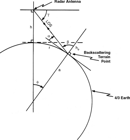
Depression angle α on a spherical earth is defined to be the complement of incidence angle β at the backscattering terrain point. Incidence angle β is the angle between the outward projection of the earth’s radius at the backscattering terrain point and the direction of illumination (or line-of-sight to the radar antenna) at the backscattering terrain point. The spherical earth has two effects in the computation of depression angle. The first effect is the effective decrease in terrain elevation of the backscattering terrain point due to the sphericity of the earth, whereby the surface of the earth (i.e., an imaginary sphere with height above mean sea level constant and equal to that of the backscattering terrain point) drops off with increasing range from the radar. This effective decrease in terrain elevation of the backscattering terrain point is denoted as he. On a spherical earth of radius a, he is computed as
Including he, the angle below the local horizontal at the radar antenna at which the backscattering terrain point is observed, denoted γ, is computed as
Angle γ is referred to as the off-axis angle. It is the angle for which elevation gain correction on the elevation pattern of the radar antenna is performed in computation of clutter strength.
The second effect of the spherical earth on depression angle is the rotation of the local Cartesian reference frame at the backscattering terrain point with respect to that at the radar antenna. This angle of rotation, denoted by φ, is computed as
That is, the correct illumination angle to be associated with the clutter measured from the backscattering terrain point is the angle α above the local horizontal at which an observer at the backscattering terrain point sees the radar, not the angle γ at which an observer at the radar sees the terrain point. Incorporating both effects, depression angle α is computed as
It is depression angle α which is computed for each clutter patch in this book and associated thereafter with the measured amplitude distribution of the clutter patch. For r < a, both α (seen by the observer at the terrain point) and γ (seen by the observer at the radar) simplify to ≈ h/r.
See [1], Section 1.11 for related discussion (N.B., the angle nomenclature in [1] differs from that utilized here; the term “grazing angle” herein means the angle between the tangent to the local terrain surface at the backscattering terrain point and the direction of illumination; [1] does not utilize or define the term “grazing angle” as used herein; “grazing angle” in [1] is equivalent to “depression angle” here, and “depression angle” in [1] is equivalent to “off-axis angle” here).
Positive h. For the majority of the clutter patches of this book, effective radar height h is positive, i.e., h > 0. For h > 0, range to the spherical earth horizon, denoted by r′, is given by ![]() . At the spherical earth horizon (i.e., r = r′), depression angle α = 0, and off-axis angle
. At the spherical earth horizon (i.e., r = r′), depression angle α = 0, and off-axis angle ![]() . Beyond the spherical earth horizon (i.e., r > r′), α is negative. That is, due to the spherical earth, at long enough ranges depression angle α becomes negative even though effective radar height h is positive. Most of the clutter patches of this book occur at ranges within the spherical earth horizon (i.e., r < r′) which, for h > 0, leads to positive values of depression angle α. However, occasional long-range clutter patches occur at ranges beyond the imaginary spherical earth horizon (i.e., r > r′), but still remain within line-of-sight visibility to the radar on the real earth. Such long-range clutter patches lead, properly, to negative values of α, even though h > 0. Such clutter patches are often weak due to diffraction loss over the long ranges of intervening terrain at near grazing incidence. Some examples of such long-range patches for urban terrain are discussed in Chapter 5.
. Beyond the spherical earth horizon (i.e., r > r′), α is negative. That is, due to the spherical earth, at long enough ranges depression angle α becomes negative even though effective radar height h is positive. Most of the clutter patches of this book occur at ranges within the spherical earth horizon (i.e., r < r′) which, for h > 0, leads to positive values of depression angle α. However, occasional long-range clutter patches occur at ranges beyond the imaginary spherical earth horizon (i.e., r > r′), but still remain within line-of-sight visibility to the radar on the real earth. Such long-range clutter patches lead, properly, to negative values of α, even though h > 0. Such clutter patches are often weak due to diffraction loss over the long ranges of intervening terrain at near grazing incidence. Some examples of such long-range patches for urban terrain are discussed in Chapter 5.
Negative h. For a significant number of the clutter patches of this book, effective radar height h is negative, i.e., h < 0. When h < 0, the terrain elevation of the clutter patch is higher than the radar antenna. To be within line-of-sight visibility in such circumstances, the terrain within the clutter patch must be of steep slope greater than the absolute value of the depression angle at which it is observed. For this reason, clutter strengths often rise quickly with increasing negative depression angle. For convenience, when h < 0, let H = −h, so that H is a positive number. Also, for ![]() . Then, when h < 0, Eq. (2.C.4) for depression angle α becomes
. Then, when h < 0, Eq. (2.C.4) for depression angle α becomes
Equation (2.C.5) indicates that α is always negative for h < 0. If the magnitude of α is represented as |α|, then Eq. (2.C.5) further indicates that, for h < 0, with increasing range r, |α| first decreases from a large value determined by H/r to a minimum value of ![]() at r = r′; and then as r continues to increase (i.e., r > r′), |α| begins to increase as r/2a. Almost all of the clutter patches of this book with h < 0 occur at ranges r < r′; that is, the negative values of depression angle associated with them are primarily the result of negative values of effective radar height h, and are only secondarily the result of the long-range spherical earth effect r/2a. This is true even for the long-range mountain patches for which results are provided in Chapter 5. Although many of the long-range mountain patches occur at ranges of 100 km or more, these mountain patches occur at elevations 4000 to 5000 ft above the prairie site elevations at which they were measured, so that their long ranges remain less than
at r = r′; and then as r continues to increase (i.e., r > r′), |α| begins to increase as r/2a. Almost all of the clutter patches of this book with h < 0 occur at ranges r < r′; that is, the negative values of depression angle associated with them are primarily the result of negative values of effective radar height h, and are only secondarily the result of the long-range spherical earth effect r/2a. This is true even for the long-range mountain patches for which results are provided in Chapter 5. Although many of the long-range mountain patches occur at ranges of 100 km or more, these mountain patches occur at elevations 4000 to 5000 ft above the prairie site elevations at which they were measured, so that their long ranges remain less than ![]() .
.
REFERENCES
1. Billingsley, J. B. “Radar ground clutter measurements and models,”. In: AGARD Conf. Proc. Target and Clutter Scattering and Their Effects on Military Radar Performance. Ottawa: ; 1991. [AGARD-CP-501, DTIC AD-P006 373. ].
2. H. C. Chan, “Radar ground clutter measurements and models, part 2: Spectral characteristics and temporal statistics,” AGARD Conference Proceedings on Target and Clutter Scattering and Their Effects on Military Radar Performance, AGARD-CP-501 (1991).
3. Anderson, J. R. “A land use and land cover classification system for use with remote sensor data,”. In: Professional Paper 964, Geological Survey. : U. S. Department of the Interior; 1975.
4. McKeague, J. A. The Canadian System of Soil Classification. In: Canadian Department of Agriculture Publ. 1646, Supply and Services. Ottawa, Canada: ; 1978.
5. Nathanson, F. E., Reilly, J. P., Cohen, M. N. Radar Design Principles, 2nd ed. New York: McGraw-Hill, 1991.
6. Skolnik, M. I. Introduction to Radar Systems, 3rd ed. New York: McGraw-Hill, 2001.
7. Long, M. W. Radar Reflectivity of Land and Sea, 3rd ed. Boston, Mass. : Artech House, 2001.
8. Hill, D. A., Wait, J. R. “Ground wave propagation over a mixed path with an elevation change,”. IEEE Trans. Ant. and Prop. January 1982; Vol. AP-30(No. 1):139–141.
9. Jao, J. K. “Amplitude distribution of composite terrain radar clutter and the. K-distribution,” IEEE Trans. Ant. Prop. October 1984; Vol. AP-32(no. 10):1049–1062.
10. Barton, D. K. “Land clutter models for radar design and analysis,”. Proc. IEEE. February 1985; Vol. 73(no. 2):198–204.
11. Sekine, M., Mao, Y. Weibull Radar Clutter. London, U. K. : Peter Peregrinus Ltd., 1990.
12. Boothe, R. R. “The Weibull Distribution Applied to the Ground Clutter Backscatter Coefficient,”. In: U. S. Army Missile Command Rept. No. RE-TR-69-15. AL: Redstone Arsenal; June 1969. [DTIC AD-691109. ].
13. Jakeman, E. “On the statistics of K-distributed noise,”. J. Physics A; Math. Gen. 1980; Vol. 13:31–48.
14. Oliver, C. J. “A model for non-Rayleigh scattering statistics,”. Opt. Acta. 1984; Vol. 31:701–722.
15. Bendat, J. S., Piersol, A. G. Random Data: Analysis and Measurement Procedures, 2nd ed. New York: Wiley, 1986.
16. Barton, D. K. Modern Radar System Analysis. Norwood, MA: Artech House, 1988.
17. Ruck, G. T., Barrick, D. E., Stuart, W. D., Krichbaum, C. K. Radar Cross Section Handbook. New York: Plenum Press, 1970; 676–679.
15.Figure 2.21 and its discussion here may be compared with Figure 1.4 and its discussion in Section 1.2.5.
16.The quantity actually provided is the percent of samples above radar noise level, which is the complement of the percent of microshadowed cells.
17.Rayleigh for ![]() ; exponential for σ°.
; exponential for σ°.
18.Also, consider the distribution of Figure 2.41 from the point-of-view of statistical estimation theory. Thus, sample size N = 448, sample mean ![]() , and sample variance σ2 = 25 dB. The rms error of
, and sample variance σ2 = 25 dB. The rms error of ![]() is
is  . Hence the quantity
 ![]() is statistically “good” to −33.0 ± 0.24 dB.
is statistically “good” to −33.0 ± 0.24 dB.
19.More precisely, if the voltage (x)1/2 is Rayleigh distributed, then the power x follows an exponential distribution in which ![]() .
.
20.If the n-th percentile level (0 ≤ n ≤ 100) occurs at ![]() in the distribution of xi, it occurs at
in the distribution of xi, it occurs at ![]() in the distribution yi, since percentile level only indicates relative position in the distribution. This is not true of moment-dependent quantities. That is, Mq(y) ≠ 10 log10 Mq (x).
in the distribution yi, since percentile level only indicates relative position in the distribution. This is not true of moment-dependent quantities. That is, Mq(y) ≠ 10 log10 Mq (x).
21.That is, voltage-like quantities are Rayleigh distributed; power-like quantities are exponentially distributed. Here, x is a power-like quantity.