
Chapter 4
Multivariate Data Analysis
Multivariate data analysis studies simultaneously several time series, but the time series properties are ignored, and thus the analysis can be called cross-sectional.
The copula is an important concept of multivariate data analysis. Copula models are a convenient way to separate multivariate analysis to the purely univariate and to the purely multivariate components. We compose a multivariate distribution into the part that describes the dependence and into the parts that describe the marginal distributions. The marginal distributions can be estimated efficiently using nonparametric methods, but it can be useful to apply parametric models to estimate dependence, for a high-dimensional distribution. Combining nonparametric estimators of marginals and a parametric estimator of the copula leads to a semiparametric estimator of the distribution.
Multivariate data can be described using such statistics as linear correlation, Spearman's rank correlation, and Kendall's rank correlation. Linear correlation is used in the Markowitz portfolio selection. Rank correlations are more natural concepts to describe dependence, because they are determined by the copula, whereas linear correlation is affected by marginal distributions. Coefficients of tail dependence can capture whether the dependence of asset returns is larger during the periods of high volatility.
Multivariate graphical tools include scatter plots, which can be combined with multidimensional scaling and other dimension reduction methods.
Section 4.1 studies measures of dependence. Section 4.2 considers multivariate graphical tools. Section 4.3 defines multivariate parametric distributions such as multivariate normal, multivariate Student, and elliptical distributions. Section 4.4 defines copulas and models for copulas.
4.1 Measures of Dependence
Random vectors ![]() are said to be independent if
are said to be independent if
for all measurable ![]() . This is equivalent to
. This is equivalent to
for all measurable ![]() , so knowledge of
, so knowledge of ![]() does not affect the probability evaluations of
does not affect the probability evaluations of ![]() . The complete dependence between random vectors
. The complete dependence between random vectors ![]() and
and ![]() occurs when there is a bijection
occurs when there is a bijection ![]() so that
so that
holds almost everywhere. When the random vectors are not independent and not completely dependent we may try to quantify the dependency between two random vectors. We may say that two random vectors have the same dependency when they have the same copula, and the copula is defined in Section 4.4.
Correlation coefficients are defined between two real valued random variables. We define three correlation coefficients: linear correlation ![]() , Spearman's rank correlation
, Spearman's rank correlation ![]() , and Kendall's rank correlation
, and Kendall's rank correlation ![]() . All of these correlation coefficients satisfy
. All of these correlation coefficients satisfy
where ![]() and
and ![]() are real valued random variables. Furthermore, if
are real valued random variables. Furthermore, if ![]() and
and ![]() are independent, then
are independent, then ![]() for any of the correlation coefficients. Converse does not hold, so that correlation zero does not imply independence.
for any of the correlation coefficients. Converse does not hold, so that correlation zero does not imply independence.
Complete dependence was defined by (4.1). Both for the Spearman's rank correlation and for the Kendall's rank correlation we have that
where ![]() or
or ![]() . In the case of real valued random variables the complete dependency can be divided into comonotonicity and countermonotonicity. Real-valued random variables
. In the case of real valued random variables the complete dependency can be divided into comonotonicity and countermonotonicity. Real-valued random variables ![]() and
and ![]() are said to be comonotonic if there is a strictly increasing function
are said to be comonotonic if there is a strictly increasing function ![]() so that
so that ![]() almost everywhere. Real-valued random variables
almost everywhere. Real-valued random variables ![]() and
and ![]() are said to be countermonotonic if there is a strictly decreasing function
are said to be countermonotonic if there is a strictly decreasing function ![]() so that
so that ![]() almost everywhere. Both for the Spearman's rank correlation and for the Kendall's rank correlation we have that
almost everywhere. Both for the Spearman's rank correlation and for the Kendall's rank correlation we have that ![]() if and only if
if and only if ![]() and
and ![]() are comonotonic, and
are comonotonic, and ![]() if and only if
if and only if ![]() and
and ![]() are countermonotonic, where
are countermonotonic, where ![]() or
or ![]() .
.
The linear correlation coefficient ![]() does not satisfy (4.2). However, we have that
does not satisfy (4.2). However, we have that
If ![]() , then
, then ![]() . If
. If ![]() , then
, then ![]() .
.
4.1.1 Correlation Coefficients
We define linear correlation ![]() , Spearman's rank correlation
, Spearman's rank correlation ![]() , and Kendall's rank correlation
, and Kendall's rank correlation ![]() .
.
4.1.1.1 Linear Correlation
The linear correlation coefficient between real valued random variables ![]() and
and ![]() is defined as
is defined as

where the covariance is
and the standard deviation is ![]() .
.
We noted in (4.3) that the linear correlation coefficient characterizes linear dependency. However, (4.2) does not hold for the linear correlation coefficient. Even when ![]() and
and ![]() are completely dependent, it can happen that
are completely dependent, it can happen that ![]() . For example, let
. For example, let ![]() ,
, ![]() , and
, and ![]() , where
, where ![]() . Then,
. Then,
and ![]() only for
only for ![]() , otherwise
, otherwise ![]() ; the example is from McNeil et al. (2005, p. 205).
; the example is from McNeil et al. (2005, p. 205).
Let us assume that ![]() and
and ![]() have continuous distributions and let us denote with
have continuous distributions and let us denote with ![]() the distribution function of
the distribution function of ![]() and with
and with ![]() and
and ![]() the marginal distribution functions. Then,
the marginal distribution functions. Then,


where ![]() ,
, ![]() , is the copula of the distribution of
, is the copula of the distribution of ![]() , as defined in (4.29). Equation (4.5) is called Höffding's formula, and its proof can be found in McNeil et al. (2005, p. 203). Thus, the linear correlation is not solely a function of the copula, it depends also on the marginal distributions
, as defined in (4.29). Equation (4.5) is called Höffding's formula, and its proof can be found in McNeil et al. (2005, p. 203). Thus, the linear correlation is not solely a function of the copula, it depends also on the marginal distributions ![]() and
and ![]() .
.
The linear correlation coefficient can be estimated with the sample correlation. Let ![]() be a sample from the distribution of
be a sample from the distribution of ![]() and
and ![]() be a sample from the distribution of
be a sample from the distribution of ![]() . The sample correlation coefficient is defined as
. The sample correlation coefficient is defined as

where ![]() and
and ![]() . An alternative estimator is defined in (4.10).
. An alternative estimator is defined in (4.10).
4.1.1.2 Spearman's Rank Correlation
Spearman's rank correlation (Spearman's rho) is defined by
where ![]() is the distribution function of
is the distribution function of ![]() ,
, ![]() . If
. If ![]() and
and ![]() have continuous distributions, then
have continuous distributions, then

where ![]() ,
, ![]() , is the copula as defined in Section 4.4 (see McNeil et al., 2005, p. 207).1 Thus, Spearman's correlation coefficient is defined solely in terms of the copula.
, is the copula as defined in Section 4.4 (see McNeil et al., 2005, p. 207).1 Thus, Spearman's correlation coefficient is defined solely in terms of the copula.
We have still another way of writing Spearman's rank correlation. Let ![]() ,
, ![]() , and
, and ![]() , let
, let ![]() have the same distribution, and let
have the same distribution, and let ![]() be independent. Then,
be independent. Then,
The sample Spearman's rank correlation can be defined as the sample linear correlation coefficient between the ranks. Let ![]() be a sample from the distribution of
be a sample from the distribution of ![]() and
and ![]() be a sample from the distribution of
be a sample from the distribution of ![]() . The rank of observation
. The rank of observation ![]() ,
, ![]() ,
, ![]() , is
, is
That is, ![]() is the number of observations of the
is the number of observations of the ![]() th variable smaller or equal to
th variable smaller or equal to ![]() .2
Let us use the shorthand notation
.2
Let us use the shorthand notation
so that ![]() ,
, ![]() . Then the sample Spearman's rank correlation can be written as
. Then the sample Spearman's rank correlation can be written as
where ![]() is the sample linear correlation coefficient, defined in (4.6). Since
is the sample linear correlation coefficient, defined in (4.6). Since ![]() and
and ![]() , we can write
, we can write

4.1.1.3 Kendall's Rank Correlation
Let ![]() and
and ![]() , let
, let ![]() and
and ![]() have the same distribution, and let
have the same distribution, and let ![]() and
and ![]() be independent. Kendall's rank correlation (Kenadall's tau) is defined by
be independent. Kendall's rank correlation (Kenadall's tau) is defined by

When ![]() and
and ![]() have continuous distributions, we have
have continuous distributions, we have
and we can write

where ![]() ,
, ![]() , is the copula as defined in Section 4.4 (see McNeil et al., 2005, p. 207).
, is the copula as defined in Section 4.4 (see McNeil et al., 2005, p. 207).
Let us define an estimator for ![]() . Let
. Let ![]() be a sample from the distribution of
be a sample from the distribution of ![]() and
and ![]() be a sample from the distribution of
be a sample from the distribution of ![]() . Kendall's rank correlation can be written as
. Kendall's rank correlation can be written as
where ![]() , if
, if ![]() and
and ![]() , if
, if ![]() . This leads to the sample version
. This leads to the sample version

The computation takes longer than for the sample linear correlation and for the sample Spearman's correlation.
4.1.1.4 Relations between the Correlation Coefficients
We have a relation between the linear correlation and the Kendall's rank correlation for the elliptical distributions. Let ![]() be a bivariate random vector. For all elliptical distributions with
be a bivariate random vector. For all elliptical distributions with ![]() ,
,
where ![]() is the Kendall's rank correlation, as defined in (4.7), and
is the Kendall's rank correlation, as defined in (4.7), and ![]() is the linear correlation, as defined in (4.4) (see McNeil et al., 2005, p. 217). This relationship can be applied to get an alternative and a more robust estimator for the estimator (4.6) of linear correlation. Define the estimator as
is the linear correlation, as defined in (4.4) (see McNeil et al., 2005, p. 217). This relationship can be applied to get an alternative and a more robust estimator for the estimator (4.6) of linear correlation. Define the estimator as
where ![]() is the estimator (4.8).
is the estimator (4.8).
For the distributions with a Gaussian copula, we also have a relation between the Spearman's rank correlation and the linear correlation. Let ![]() be a distribution with a Gaussian copula and continuous margins. Then,
be a distribution with a Gaussian copula and continuous margins. Then,
and (4.9) holds also (see McNeil et al., 2005, p. 215).
Figure 4.1 studies linear correlation and Spearman's rank correlation for S&P 500 and Nasdaq-100 daily data, described in Section 2.4.2. Panel (a) shows a moving average estimate of linear correlation (blue) and Spearman's rank correlation (yellow). We use the one-sided moving average defined as

where ![]() are the S&P 500 centered returns and
are the S&P 500 centered returns and ![]() are the Nasdaq-100 centered returns. The weights
are the Nasdaq-100 centered returns. The weights ![]() are one for the last 500 observations, and zero for the other observations. See (6.5) for a more general moving average. The moving average estimator
are one for the last 500 observations, and zero for the other observations. See (6.5) for a more general moving average. The moving average estimator ![]() is the Spearman's rho computed from the 500 previous observations. Panel (b) shows the correlation coefficients together with the moving average estimates of the standard deviation of S&P 500 returns (solid black line) and Nasdaq-100 returns (dashed black line). All time series are scaled to take values in the interval
is the Spearman's rho computed from the 500 previous observations. Panel (b) shows the correlation coefficients together with the moving average estimates of the standard deviation of S&P 500 returns (solid black line) and Nasdaq-100 returns (dashed black line). All time series are scaled to take values in the interval ![]() . We see that there is some tendency that the inter-stock correlations increase in volatile periods.
. We see that there is some tendency that the inter-stock correlations increase in volatile periods.

Figure 4.1 Linear and Spearman's correlation, together with volatility. (a) Time series of moving average estimates of correlation between S&P 500 and Nasdaq-100 returns, with linear correlation (blue) and Spearman's rho (yellow); (b) we have added moving average estimates of the standard deviation of S&P 500 (black solid) and Nasdaq-100 (black dashed).
4.1.2 Coefficients of Tail Dependence
The coefficient of upper tail dependence is defined for random variables ![]() and
and ![]() with distribution functions
with distribution functions ![]() and
and ![]() as
as
where ![]() and
and ![]() are the generalized inverses. Similarly, the coefficient of lower tail dependence is
are the generalized inverses. Similarly, the coefficient of lower tail dependence is
See McNeil et al. (2005, p. 209).
4.1.2.1 Tail Coefficients in Terms of the Copula
The coefficients of upper and lower tail dependence can be defined in terms of the copula. Let ![]() and
and ![]() be continuous. We have that
be continuous. We have that

Also,
Thus, the coefficient of upper tail dependence is

We have that
Also,
Thus, the coefficient of lower tail dependence for continuous ![]() and
and ![]() is equal to
is equal to
4.1.2.2 Estimation of Tail Coefficients
Equations (4.11) and (4.12) suggest estimators for the coefficients of tail dependence. We can estimate the upper tail coefficient nonparametrically, using

where ![]() is the empirical copula, defined in (4.38), and
is the empirical copula, defined in (4.38), and ![]() is close to 1. We can take, for example,
is close to 1. We can take, for example, ![]() , where
, where ![]() . The coefficient of lower tail dependence can be estimated by
. The coefficient of lower tail dependence can be estimated by

where ![]() is close to zero. We can take, for example,
is close to zero. We can take, for example, ![]() , where
, where ![]() . These estimators have been studied in Dobric and Schmid (2005), Frahm et al. (2005), and Schmidt and Stadtmüller (2006).
. These estimators have been studied in Dobric and Schmid (2005), Frahm et al. (2005), and Schmidt and Stadtmüller (2006).
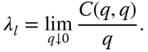
Figure 4.2 studies tail coefficients for S&P 500 and Nasdaq-100 daily data, described in Section 2.4.2. Panel (a) shows the tail coefficients as a function of ![]() for lower tail coefficients (red) and as a function of
for lower tail coefficients (red) and as a function of ![]() for upper tail coefficients (blue). Panel (b) shows a moving average estimate of the lower tail coefficients. The tail coefficient is estimated using the window of the latest 1000 observations, for
for upper tail coefficients (blue). Panel (b) shows a moving average estimate of the lower tail coefficients. The tail coefficient is estimated using the window of the latest 1000 observations, for ![]() .
.
Figure 4.2 Tail coefficients for S&P 500 and Nasdaq-100 returns. (a) Tail coefficients as a function of  for lower tail coefficients (red) and as a function of
  for upper tail coefficients (blue); (b) time series of moving average estimates of lower tail coefficients.
4.1.2.3 Tail Coefficients for Parametric Families
The coefficients of lower and upper tail dependence for the Gaussian distributions are zero. The coefficients of lower and upper tail dependence for the Student distributions with degrees of freedom ![]() and correlation coefficient
and correlation coefficient ![]() are
are

where ![]() is the distribution function of the univariate
is the distribution function of the univariate ![]() -distribution with
-distribution with ![]() degrees of freedom, and we assume that
degrees of freedom, and we assume that ![]() ; see McNeil et al. (2005, p. 211).
; see McNeil et al. (2005, p. 211).
4.2 Multivariate Graphical Tools
First, we describe scatter plots and smooth scatter plots. Second, we describe visualization of correlation matrices with multidimensional scaling.
4.2.1 Scatter Plots
A two-dimensional scatter plot is a plot of points ![]() .
.
Figure 4.3 shows scatter plots of daily net returns of S&P 500 and Nasdaq-100. The data is described in Section 2.4.2. Panel (a) shows the original data and panel (b) shows the corresponding scatter plot after copula preserving transform with standard normal marginals, as defined in (4.36).

Figure 4.3 Scatter plots. Scatter plots of the net returns of S&P 500 and Nasdaq-100. (a) Original data; (b) copula transformed data with marginals being standard normal.
When the sample size is large, then the scatter plot is mostly black, so the visuality of density of the points in different regions is obscured. In this case it is possible to use histograms to obtain a smooth scatter plot. A multivariate histogram is defined in (3.42). First we take square roots ![]() of the bin counts
of the bin counts ![]() and then we define
and then we define ![]() . Now
. Now ![]() . Values
. Values ![]() close to one are shown in light gray, and values
close to one are shown in light gray, and values ![]() close to zero are shown in dark gray. See Carr et al. (1987) for a study of histogram plotting.
close to zero are shown in dark gray. See Carr et al. (1987) for a study of histogram plotting.
Figure 4.4 shows smooth scatter plots of daily net returns of S&P 500 and Nasdaq-100. The data is described in Section 2.4.2. Panel (a) shows a smooth scatter plot of the original data and panel (b) shows the corresponding scatter plot after copula preserving transform when the marginals are standard Gaussian.

Figure 4.4 Smooth scatter plots. Scatter plots of the net returns of S&P 500 and Nasdaq-100. (a) Original data; (b) copula transformed data with marginals being standard normal.
4.2.2 Correlation Matrix: Multidimensional Scaling
First, we define the correlation matrix. Second, we show how the correlation matrix may be visualized using multidimensional scaling.
4.2.2.1 Correlation Matrix
The correlation matrix is the ![]() matrix whose elements are the linear correlation coefficients
matrix whose elements are the linear correlation coefficients ![]() for
for ![]() . The sample correlation matrix is the matrix whose elements are the sample linear correlation coefficients.
. The sample correlation matrix is the matrix whose elements are the sample linear correlation coefficients.
The correlation matrix can be defined using matrix notation. The covariance matrix of random vector ![]() is defined by
is defined by
The covariance matrix is the ![]() matrix whose elements are
matrix whose elements are ![]() for
for ![]() , where we denote
, where we denote ![]() . Let
. Let
be the diagonal matrix whose diagonal is the vector of the inverses of the standard deviations. Then the correlation matrix is
The covariance matrix can be estimated by the sample covariance matrix

where ![]() are identically distributed observations whose distribution is the same as the distribution of
are identically distributed observations whose distribution is the same as the distribution of ![]() , and
, and ![]() is the arithmetic mean.
is the arithmetic mean.
4.2.2.2 Multidimensional Scaling
Multidimensional scaling makes a nonlinear mapping of data ![]() to
to ![]() , or to any space
, or to any space ![]() with
with ![]() . We can define the mapping
. We can define the mapping ![]() of multidimensional scaling in two steps:
of multidimensional scaling in two steps:
- 1. Compute the pairwise distances
 ,
,  .
. - 2. Find points
 so that
  for
for  .
.
In practice, we may not be able to find a mapping that preserves the distances exactly, but we find a mapping ![]() so that the stress functional
so that the stress functional
is minimized. Sammon's mapping uses the stress functional

This stress functional emphasizes small distances. Numerical minimization is needed to solve the minimization problems.
Multidimensional scaling can be used to visualize correlations between time series. Let ![]() be the time series of returns of company
be the time series of returns of company ![]() , where
, where ![]() . When we normalize the time series of returns so that the vector of returns has sample mean zero and sample variance one, then the Euclidean distance is equivalent to using the correlation distance. Indeed, let
. When we normalize the time series of returns so that the vector of returns has sample mean zero and sample variance one, then the Euclidean distance is equivalent to using the correlation distance. Indeed, let

where ![]() and
and ![]() . Now
. Now
where ![]() is the sample linear correlation. Thus, we apply the multidimensional scaling for the norm
is the sample linear correlation. Thus, we apply the multidimensional scaling for the norm

which is obtained by dividing the Euclidean norm by ![]() . Since
. Since
we have that
Zero correlation gives ![]() , positive correlations give
, positive correlations give ![]() , and negative correlations give
, and negative correlations give ![]() .
.
Figure 4.5 studies correlations of the returns of the components of DAX 30. We have daily observations of the components of DAX 30 starting at January 02, 2003 and ending at May 20, 2014, which makes 2892 observations. Panel (a) shows the correlation matrix as an image. We have used R-function “image.” Panel (b) shows the correlations with multidimensional scaling. We have used R-function “cmdscale.” The image of the correlation matrix is not as helpful as the multidimensional scaling. For example, we see that the return time series of Volkswagen with the ticker symbol “VOW” is an outlier. The returns of Fresenius and Fresenius Medical Care (“FRE” and “FME”) are highly correlated.

Figure 4.5 Correlations of DAX 30. (a) An image of the correlation matrix for DAX 30; (b) correlations for DAX 30 with multidimensional scaling.
4.3 Multivariate Parametric Models
We give examples of multivariate parametric models. The examples include Gaussian and Student distributions (![]() -distributions). More general families are normal variance mixture distributions and elliptical distributions.
-distributions). More general families are normal variance mixture distributions and elliptical distributions.
4.3.1 Multivariate Gaussian Distributions
A ![]() -dimensional Gaussian distribution can be parametrized with the expectation vector
-dimensional Gaussian distribution can be parametrized with the expectation vector ![]() and the
and the ![]() covariance matrix
covariance matrix ![]() . When random vector
. When random vector ![]() follows the Gaussian distribution with parameters
follows the Gaussian distribution with parameters ![]() and
and ![]() , then we write
, then we write ![]() or
or ![]() . We say that a Gaussian distribution is the standard Gaussian distribution when
. We say that a Gaussian distribution is the standard Gaussian distribution when ![]() and
and ![]() . The density function of the Gaussian distribution is
. The density function of the Gaussian distribution is
where ![]() and
and ![]() is the determinant of
is the determinant of ![]() . The characteristic function of the Gaussian distribution is
. The characteristic function of the Gaussian distribution is
where ![]() .
.
A linear transformation of a Gaussian random vector follows a Gaussian distribution: When ![]() ,
, ![]() is
is ![]() matrix, and
matrix, and ![]() is a
is a ![]() vector, then
vector, then
Also, when ![]() and
and ![]() are independent, then
are independent, then
Both of these facts can be proved using the characteristic function.3
4.3.2 Multivariate Student Distributions
A ![]() -dimensional Student distribution (
-dimensional Student distribution (![]() -distribution) is parametrized with degrees of freedom
-distribution) is parametrized with degrees of freedom ![]() , the expectation vector
, the expectation vector ![]() , and the
, and the ![]() positive definite symmetric matrix
positive definite symmetric matrix ![]() . When random vector
. When random vector ![]() follows the
follows the ![]() -distribution with parameters
-distribution with parameters ![]() ,
, ![]() , and
, and ![]() , then we write
, then we write ![]() or
or ![]() . The density function of the multivariate
. The density function of the multivariate ![]() -distribution is
-distribution is
where

The multivariate Student distributed random vector has the covariance matrix
when ![]() .
.
When ![]() , then the Student density approaches a Gaussian density. Indeed,
, then the Student density approaches a Gaussian density. Indeed, ![]() , as
, as ![]() , since
, since ![]() , when
, when ![]() . The Student density has tails
. The Student density has tails ![]() , as
, as ![]() .
.
Figure 4.6 compares multivariate Gaussian and Student densities. Panel (a) shows the Gaussian density with marginal standard deviations equal to one and correlation 0.5. Panel (b) shows the density of ![]() -distribution with degrees of freedom 2 and correlation 0.5. The density contours are in both cases ellipses but the Student density has heavier tails.
-distribution with degrees of freedom 2 and correlation 0.5. The density contours are in both cases ellipses but the Student density has heavier tails.

Figure 4.6 Gaussian and Student densities. (a) Contour plot of the Gaussian density with marginal standard deviations equal to one and correlation 0.5; (b) Student density with degrees of freedom 2 and correlation 0.5.
4.3.3 Normal Variance Mixture Distributions
Random vector ![]() follows a Gaussian distribution with parameters
follows a Gaussian distribution with parameters ![]() and
and ![]() when
when ![]() for a
for a ![]() matrix
matrix ![]() and
and
where ![]() follows the standard Gaussian distribution. This leads to the definition of a normal variance mixture distribution. We say that
follows the standard Gaussian distribution. This leads to the definition of a normal variance mixture distribution. We say that ![]() follows a normal variance mixture distribution when
follows a normal variance mixture distribution when
where ![]() follows the standard Gaussian distribution, and
follows the standard Gaussian distribution, and ![]() is a random variable independent of
is a random variable independent of ![]() . It holds that
. It holds that
and
where ![]() . When random vector
. When random vector ![]() follows the normal variance mixture distribution with parameters
follows the normal variance mixture distribution with parameters ![]() ,
, ![]() , and
, and ![]() , where
, where ![]() is the distribution function on
is the distribution function on ![]() , then we write
, then we write ![]() .
.
The density function can be calculated as

where ![]() is the density of
is the density of ![]() ,
, ![]() is the density of
is the density of ![]() ,
, ![]() is the density of
is the density of ![]() conditional on
conditional on ![]() , and
, and ![]() is defined by
is defined by

The characteristic function is obtained, using (4.16), as

where ![]() .
.
The family of normal variance mixtures ![]() is closed under linear transformations: When
is closed under linear transformations: When ![]() ,
, ![]() is
is ![]() matrix, and
matrix, and ![]() is a
is a ![]() vector, then
vector, then
This can be seen using the characteristic function, similarly as in (4.17).
Let ![]() be such random variable that
be such random variable that ![]() follows the
follows the ![]() -distribution with degrees of freedom
-distribution with degrees of freedom ![]() . Then the normal variance mixture distribution is the multivariate
. Then the normal variance mixture distribution is the multivariate ![]() -distribution
-distribution ![]() , where
, where ![]() , as defined in Section 4.3.2.
, as defined in Section 4.3.2.
4.3.4 Elliptical Distributions
The density function of an elliptical distribution has the form
where ![]() is called the density generator,
is called the density generator, ![]() is a symmetric positive definite
is a symmetric positive definite ![]() matrix, and
matrix, and ![]() . Since
. Since ![]() is positive definite, it has inverse
is positive definite, it has inverse ![]() that is positive definite, which means that for all
that is positive definite, which means that for all ![]() ,
, ![]() . Thus,
. Thus, ![]() needs to be defined only on the nonnegative real axis. Let
needs to be defined only on the nonnegative real axis. Let ![]() be such that
be such that ![]() . Then
. Then ![]() is a density generator when
is a density generator when ![]() is chosen by
is chosen by

where ![]() . We give examples of density generators.
. We give examples of density generators.
- 1. From (4.15) we see that the Gaussian distributions are elliptical and the Gaussian density generator is
4.25

- where
 .
. - 2. From (4.20) we see that the normal variance mixture distributions are elliptical and the normal variance mixture density generator is given in (4.21).
- 3. From (4.18) we see that the
 -distributions are elliptical and the Student density generator is
4.26
-distributions are elliptical and the Student density generator is
4.26
- where
 is the degrees of freedom, and
  is defined in (4.19). The Student density generator has tails
  , as
, as  , and thus the density function is integrable when
  , according to (4.24).
Let ![]() , where
, where ![]() is a
is a ![]() matrix and let
matrix and let
where ![]() follows a spherical distribution with density
follows a spherical distribution with density ![]() . Then
. Then ![]() follows an elliptical distribution with density (4.23). When random vector
follows an elliptical distribution with density (4.23). When random vector ![]() follows the elliptical distribution with parameters
follows the elliptical distribution with parameters ![]() ,
, ![]() , and
, and ![]() , where
, where ![]() is the distribution function on
is the distribution function on ![]() , then we write
, then we write ![]() . The family of elliptical distributions is closed under linear transformations: When
. The family of elliptical distributions is closed under linear transformations: When ![]() ,
, ![]() is a
is a ![]() matrix, and
matrix, and ![]() is a
is a ![]() vector, then
vector, then
This can be seen using the characteristic function, similarly as in (4.17).
4.4 Copulas
We can decompose a multivariate distribution into a part that describes the dependence and into parts that describe the marginal distributions. This decomposition helps to estimate and analyze multivariate distributions, and it helps to construct new parametric and semiparametric models for multivariate distributions.
The distribution function ![]() of random vector
of random vector ![]() is defined by
is defined by
where ![]() . The distribution functions
. The distribution functions ![]() , …,
, …, ![]() of the marginal distributions are defined by
of the marginal distributions are defined by
where ![]() .
.
A copula is a distribution function ![]() whose marginal distributions are the uniform distributions on
whose marginal distributions are the uniform distributions on ![]() . Often it is convenient to define a copula as a distribution function
. Often it is convenient to define a copula as a distribution function ![]() whose marginal distributions are the standard normal distributions. Any distribution function
whose marginal distributions are the standard normal distributions. Any distribution function ![]() may be written as
may be written as
where ![]() ,
, ![]() , are the marginal distribution functions and
, are the marginal distribution functions and ![]() is a copula. In this sense we can decompose a distribution into a part that describes only the dependence and into parts that describe the marginal distributions.
is a copula. In this sense we can decompose a distribution into a part that describes only the dependence and into parts that describe the marginal distributions.
We show in (4.29) how to construct a copula of a multivariate distribution and in (4.31) how to construct a multivariate distribution function from a copula and marginal distribution functions. We restrict ourselves to the case of continuous marginal distribution functions. These constructions were given in Sklar (1959), who considered also the case of noncontinuous margins. For notational convenience we give the formulas for the case ![]() . The generalization to the cases
. The generalization to the cases ![]() is straightforward.
is straightforward.
4.4.1 Standard Copulas
We use the term “standard copula,” when the marginals of the copula have the uniform distributions on ![]() . Otherwise, we use the term “nonstandard copula.”
. Otherwise, we use the term “nonstandard copula.”
4.4.1.1 Finding the Copula of a Multivariate Distribution
Let ![]() and
and ![]() be real valued random variables with distribution functions
be real valued random variables with distribution functions ![]() and
and ![]() . Let
. Let ![]() be the distribution function of
be the distribution function of ![]() , and assume that
, and assume that ![]() and
and ![]() are continuous. Then,
are continuous. Then,

where

and ![]() . We call
. We call ![]() in (4.29) the copula of the joint distribution of
in (4.29) the copula of the joint distribution of ![]() and
and ![]() . Copula
. Copula ![]() is the distribution function of the vector
is the distribution function of the vector ![]() ,
, ![]() , and
, and ![]() and
and ![]() are uniformly distributed random variables.4
are uniformly distributed random variables.4
The copula density is

because ![]() , where
, where ![]() is the density of
is the density of ![]() and
and ![]() and
and ![]() are the densities of
are the densities of ![]() and
and ![]() , respectively.
, respectively.
4.4.1.2 Constructing a Multivariate Distribution from a Copula
Let ![]() be a copula, that is, it is a distribution function whose marginal distributions are uniform on
be a copula, that is, it is a distribution function whose marginal distributions are uniform on ![]() . Let
. Let ![]() and
and ![]() be univariate distribution functions of continuous distributions. Define
be univariate distribution functions of continuous distributions. Define ![]() by
by
Then ![]() is a distribution function whose marginal distributions are given by distribution functions
is a distribution function whose marginal distributions are given by distribution functions ![]() and
and ![]() . Indeed, Let
. Indeed, Let ![]() be a random vector with distribution function
be a random vector with distribution function ![]() . Then,
. Then,

and ![]() for
for ![]() , because
, because ![]() .5
.5
4.4.2 Nonstandard Copulas
Typically a copula is defined as a distribution function with uniform marginals. However, we can define a copula so that the marginal distributions of the copula is some other continuous distribution than the uniform distribution on ![]() . It turns out that we get simpler copulas by choosing the marginal distributions of a copula to be the standard Gaussian distribution.
. It turns out that we get simpler copulas by choosing the marginal distributions of a copula to be the standard Gaussian distribution.
As in (4.28) we can write distribution function ![]() as
as
where ![]() is the distribution function of the standard Gaussian distribution and
is the distribution function of the standard Gaussian distribution and

![]() . Now
. Now ![]() is a distribution function whose marginals are standard Gaussians, because
is a distribution function whose marginals are standard Gaussians, because ![]() follow the uniform distribution on
follow the uniform distribution on ![]() and thus
and thus ![]() follow the standard Gaussian distribution.
follow the standard Gaussian distribution.
Conversely, given a distribution function ![]() with the standard Gaussian marginals, and univariate distribution functions
with the standard Gaussian marginals, and univariate distribution functions ![]() and
and ![]() , we can define a distribution function
, we can define a distribution function ![]() with marginals
with marginals ![]() and
and ![]() by the formula
by the formula
The copula density is

where ![]() is the density of
is the density of ![]() ,
, ![]() and
and ![]() are the densities of
are the densities of ![]() and
and ![]() , respectively, and
, respectively, and ![]() is the density of the standard Gaussian distribution.
is the density of the standard Gaussian distribution.
4.4.3 Sampling from a Copula
We do not have observations directly from the distribution of the copula but we show how to transform the sample so that we get a pseudo sample from the copula. Scatter plots of the pseudo sample can be used to visualize the copula. The pseudo sample can also be used in the maximum likelihood estimation of the copula. Before defining the pseudo sample, we show how to generate random variables from a copula.
4.4.3.1 Simulation from a Copula
Let random vector ![]() have a continuous distribution. Let
have a continuous distribution. Let  ,
, ![]() , be the distribution functions of the margins of
, be the distribution functions of the margins of ![]() . Now
. Now
is a random vector whose marginal distributions are uniform on ![]() . The distribution function of this random vector is the copula of the distribution of
. The distribution function of this random vector is the copula of the distribution of ![]() . Thus, if we can generate a random vector
. Thus, if we can generate a random vector ![]() with distribution
with distribution ![]() , we can use the rule (4.34) to generate a random vector
, we can use the rule (4.34) to generate a random vector ![]() whose distribution is the copula of
whose distribution is the copula of ![]() . Often the copula with uniform marginals is inconvenient due to boundary effects. We may get statistically more tractable distribution by defining
. Often the copula with uniform marginals is inconvenient due to boundary effects. We may get statistically more tractable distribution by defining
where ![]() is the distribution function of the standard Gaussian distribution. The components of
is the distribution function of the standard Gaussian distribution. The components of ![]() have the standard Gaussian distribution.
have the standard Gaussian distribution.
4.4.3.2 Transforming the Sample
Let us have data ![]() and denote
and denote ![]() . Let the rank of observation
. Let the rank of observation ![]() ,
, ![]() ,
, ![]() , be
, be
That is, ![]() is the number of observations of the
is the number of observations of the ![]() th variable smaller or equal to
th variable smaller or equal to ![]() . We normalize the ranks to get observations on
. We normalize the ranks to get observations on ![]() :
:

for ![]() . Now
. Now ![]() for
for ![]() . In this sense we can consider the observations as a sample from a distribution whose margins are uniform distributions on
. In this sense we can consider the observations as a sample from a distribution whose margins are uniform distributions on ![]() . Often the standard Gaussian distribution is more convenient and we define
. Often the standard Gaussian distribution is more convenient and we define

for ![]() .
.
4.4.3.3 Transforming the Sample by Estimating the Margins
We can transform the data ![]() using estimates of the marginal distributions. Let
using estimates of the marginal distributions. Let ![]() and
and ![]() be estimates of the marginal distribution functions
be estimates of the marginal distribution functions ![]() and
and ![]() , respectively. We define the pseudo sample as
, respectively. We define the pseudo sample as
where ![]() . The estimates
. The estimates ![]() and
and ![]() can be parametric estimates. For example, assuming that the
can be parametric estimates. For example, assuming that the ![]() th marginal distribution is a normal distribution, we would take
th marginal distribution is a normal distribution, we would take ![]() , where
, where ![]() is the distribution function of the standard normal distribution,
is the distribution function of the standard normal distribution, ![]() is the sample mean of
is the sample mean of ![]() , and
, and ![]() is the sample standard deviation. If
is the sample standard deviation. If ![]() are the empirical distribution functions
are the empirical distribution functions

then we get almost the same transformation as (4.35), but ![]() is now replaced by
is now replaced by ![]() :
:

4.4.3.4 Empirical Copula
The empirical distribution function ![]() is calculated using a sample
is calculated using a sample ![]() of identically distributed observations, and we define
of identically distributed observations, and we define

where we denote ![]() .
.
The empirical copula is defined similarly as the empirical distribution function. Now,

where ![]() are defined in (4.37).
are defined in (4.37).
4.4.3.5 Maximum Likelihood Estimation
Pseudo samples are needed in maximum likelihood estimation. In maximum likelihood estimation we assume that the copula has a parametric form. For example, the copula of the normal distribution, given in (4.39), is parametrized with the correlation matrix, which contains ![]() parameters. Let
parameters. Let ![]() be the copula with parameter
be the copula with parameter ![]() . The corresponding copula density is
. The corresponding copula density is ![]() , as given in (4.30). Let us have independent and identically distributed observations
, as given in (4.30). Let us have independent and identically distributed observations ![]() from the distribution of
from the distribution of ![]() . We calculate the pseudo sample
. We calculate the pseudo sample ![]() using (4.35) or (4.37). A maximum likelihood estimate is a value
using (4.35) or (4.37). A maximum likelihood estimate is a value ![]() maximizing
maximizing

over ![]() .
.
4.4.4 Examples of Copulas
We give examples of parametric families of copulas. The examples include the Gaussian copulas and the Student copulas.
4.4.4.1 The Gaussian Copulas
Let ![]() be a
be a ![]() -dimensional Gaussian random vector, as defined in Section 4.3.1. The copula of
-dimensional Gaussian random vector, as defined in Section 4.3.1. The copula of ![]() is
is
where ![]() is the distribution function of
is the distribution function of ![]() distribution,
distribution, ![]() is the correlation matrix of
is the correlation matrix of ![]() , and
, and ![]() is the distribution function of
is the distribution function of ![]() distribution.
distribution.
Indeed, let us denote ![]() , where
, where ![]() is the standard deviation of
is the standard deviation of ![]() . Then
. Then ![]() follows the distribution
follows the distribution ![]() .6 Let
.6 Let ![]() be the distribution function of
be the distribution function of ![]() . Then, using the notation
. Then, using the notation ![]() ,
,

where ![]() . Also,7
. Also,7
for ![]() . Thus,
. Thus,
Figure 4.7 shows perspective plots of the densities of the Gaussian copula. The margins are uniform on ![]() . The correlation parameter is in panel (a)
. The correlation parameter is in panel (a) ![]() and in panel (b)
and in panel (b) ![]() . Figure 4.7 shows that the perspective plots of the copula densities are not intuitive, because the probability mass is concentrated near the corners of the square
. Figure 4.7 shows that the perspective plots of the copula densities are not intuitive, because the probability mass is concentrated near the corners of the square ![]() , especially when the correlation is high. From now on we will show only pictures of copulas with standard Gaussian margins, as defined in (4.32), because these give more intuitive representation of the copula.
, especially when the correlation is high. From now on we will show only pictures of copulas with standard Gaussian margins, as defined in (4.32), because these give more intuitive representation of the copula.

Figure 4.7 Gaussian copulas. Perspective plots of the densities of the Gaussian copula with the correlation (a)  and (b)
  . The margins are uniform on
  .
.
4.4.4.2 The Student Copulas
Let ![]() be a
be a ![]() -dimensional
-dimensional ![]() -distributed random vector, as defined in Section 4.3.2. The copula of
-distributed random vector, as defined in Section 4.3.2. The copula of ![]() is
is
where ![]() is the distribution function of
is the distribution function of ![]() distribution,
distribution, ![]() is the correlation matrix of
is the correlation matrix of ![]() , and
, and ![]() is the distribution function of the univariate
is the distribution function of the univariate ![]() -distribution with degrees of freedom
-distribution with degrees of freedom ![]() .
.
Indeed, the claim follows similarly as in the Gaussian case for
where ![]() and
and ![]() is the square root of the
is the square root of the ![]() th element in the diagonal of
th element in the diagonal of ![]() . The matrix
. The matrix ![]() is indeed the correlation matrix, since
is indeed the correlation matrix, since
where ![]() ,
, ![]() .
.
Figure 4.8 shows contour plots of the densities of the Student copula when the margins are standard Gaussian. The correlation is ![]() . The degrees of freedom are in panel (a) two and in panel (b) four. The Gaussian and Student copulas are similar in the main part of the distribution but they differ in the tails (in the corners of the unit square). The Gaussian copula has independent extremes (asymptotic tail independence) but the Student copula generates concomitant extremes with a nonzero probability. The probability of concomitant extremes is larger when the degrees of freedom is smaller and the correlation coefficient is larger.
. The degrees of freedom are in panel (a) two and in panel (b) four. The Gaussian and Student copulas are similar in the main part of the distribution but they differ in the tails (in the corners of the unit square). The Gaussian copula has independent extremes (asymptotic tail independence) but the Student copula generates concomitant extremes with a nonzero probability. The probability of concomitant extremes is larger when the degrees of freedom is smaller and the correlation coefficient is larger.

Figure 4.8 Student copula with standard Gaussian margins. Contour plots of the densities of the Student copula with degrees of freedom (a) 2 and (b) 4. The correlation is  .
.
4.4.4.3 Other Copulas
We define Gumbel and Clayton copulas. These are examples of Archimedean copulas. Gaussian and Student copulas are examples of elliptical copulas.
The Gumbel–Hougaard Copulas
The Gumbel–Hougaard or the Gumbel family of copulas is defined by

where ![]() is the parameter. When
is the parameter. When ![]() , then
, then ![]() and when
and when ![]() , then
, then ![]() .
.
Figure 4.9 shows contour plots of the densities with the Gumbel copula when ![]() ,
, ![]() , and
, and ![]() . The marginals are standard Gaussian.
. The marginals are standard Gaussian.

Figure 4.9 Gumbel copula. Contour plots of the densities of the Gumbel copula with  ,
,  , and
, and  . The marginals are standard Gaussian.
The Clayton Copulas
Clayton's family of copulas is defined by

where ![]() . When
. When ![]() , we define
, we define ![]() . When the parameter
. When the parameter ![]() increases, then the dependence between coordinate variables increases. The dependence is larger in the negative orthant. The Clayton family was discussed in Clayton (1978).
increases, then the dependence between coordinate variables increases. The dependence is larger in the negative orthant. The Clayton family was discussed in Clayton (1978).
Figure 4.10 shows contour plots of the densities with the Clayton copula when ![]() ,
, ![]() , and
, and ![]() . The marginals are standard Gaussian.
. The marginals are standard Gaussian.

Figure 4.10 Clayton copula. Contour plots of the densities of the Clayton copula with  ,
,  , and
, and  . The marginals are standard Gaussian.
Elliptical Copulas
Elliptical distributions are defined in Section 4.3.4. An elliptical copula is obtained from an elliptical distribution ![]() by the construction (4.29). The Gaussian copula and the Student copula are elliptical copulas.
by the construction (4.29). The Gaussian copula and the Student copula are elliptical copulas.
Archimedean Copulas
Archimedean copulas have the form
where ![]() is strictly decreasing, continuous, convex, and
is strictly decreasing, continuous, convex, and ![]() . For
. For ![]() to be a copula, we need that
to be a copula, we need that ![]() ,
, ![]() . The function
. The function ![]() is called the generator. The product copula, Gumbel copula, Clayton copula, and Frank copula are all Archimedean copulas and we have:
is called the generator. The product copula, Gumbel copula, Clayton copula, and Frank copula are all Archimedean copulas and we have:
- product copula:
 ,
, - Gumbel copula:
 ,
, - Clayton copula:
 ,
, - Frank copula:
 .
.
The density of an Archimedean copula is
where ![]() is the second derivative of
is the second derivative of ![]() :
:

because ![]() . We have:
. We have:
- Gumbel copula:
 ,
,  ,
,  ,
, - Clayton copula:
 ,
,  ,
,  ,
, - Frank copula:
 ,
,  ,
,  .
.
4.4.4.4 Empirical Results
Research on testing the hypothesis of Gaussian copula and other copulas on financial data has been done in Malevergne and Sornette (2003), and summarized in Malevergne and Sornette (2005). They found that the Student copula is a good model for foreign exchange rates but for the stock returns the situation is not clear.
Patton (2005) takes into account the volatility clustering phenomenon. He filters the marginal data by a GARCH process and shows that the conditional dependence structure between Japanese Yen and Euro is better described by Clayton's copula than by the Gaussian copula. Note, however, that the copula of the residuals is not the same as the copula of the raw returns and many filters can be used (ARCH, GARCH, and multifractal random walk). Using the multivariate multifractal filter of Muzy et al. (2001) leads to a nearly Gaussian copula.
Breymann et al. (2003) show that the daily returns of German Mark/Japanese Yen are best described by a Student copula with about six degrees of freedom, when the alternatives are the Gaussian, Clayton's, Gumbel's, and Frank's copulas. The Student copula seems to provide an even better description for returns at smaller time scales, when the time scale is larger than 2 h. The best degrees of freedom is four for the 2-h scale.
Mashal and Zeevi (2002) claim that the dependence between stocks is better described by a Student copula with 11–12 degrees of freedom than by a Gaussian copula.


where ![]() is the characteristic function of
is the characteristic function of ![]() .
.