
Chapter 9
Some Basic Concepts of Portfolio Theory
Portfolio theory studies two related problems: (1) how to construct a portfolio with desirable properties and (2) how to evaluate the performance of a portfolio. In this chapter, we concentrate on the concepts related to the construction of portfolios. A portfolio is constructed by allocating the available wealth among some basic assets. The return of a portfolio is a weighted average of the returns of the basic assets, the weights expressing the proportion of wealth allocated to each basic assets. There exist also portfolios that require zero initial wealth. Such portfolios are constructed using borrowing or option writing.
A main topic of the chapter is to introduce concepts related to the comparison of return and wealth distributions, and this topic is addressed in Section 9.2. In order to study portfolio construction we need to define what it means that a wealth distribution or a return distribution is better than another such distribution. (Here wealth distribution means the probability distribution of wealth, when wealth is considered as a random variable, and we do not mean the distribution of wealth in the sense of allocation of wealth among different people.) In portfolio selection we try to select the weights of basic assets so that the distribution of the return of the portfolio is in some sense optimal.
The optimal distribution of the return is such that the expected return is high but the risk of negative returns is small. The expected return of a portfolio is determined by the expected returns of the basic assets, but the risk of the return distribution depends on the joint distribution of the returns of the basic assets. The two main ways to compare returns is the use of the mean–variance criterion and the use of the expected utility.
The issue of multiperiod portfolio selection is an important and interesting research topic. However, we do not address this topic in any depth, but only in Section 9.3. The bypassing of multiperiod portfolio selection can be justified by the fact that for the logarithmic utility function there is no difference between the one period and multiperiod portfolio selection. Thus, when we ignore the effect of varying risk aversion and restrict ourselves to the logarithmic utility, then we can ignore the issues related to multiperiod portfolio selection. Note that we discuss certain aspects of multiperiod portfolio in the connection of pricing of options, because prices of options are related to the initial wealth of a trading strategy, which approximately replicates the payoff of the option.
Section 9.1 discusses some basic concepts related to portfolios and their returns. These concepts include the concept of a trading strategy, wealth process, self-financing, portfolio weight, shorting, and leveraging. Section 9.2 discusses the comparison of return and wealth distributions. Section 9.3 discusses issues related to multiperiod portfolio selection.
9.1 Portfolios and Their Returns
The components of a portfolio can be stocks, bonds, commodities, currencies, or other financial assets. The risk-free bond (bank account) can also be included in the portfolio. The price of the risk-free bond is denoted by ![]() . Let us have
. Let us have ![]() risky portfolio components and let
risky portfolio components and let
be the vector of the prices of the risky portfolio components at time ![]() . Prices satisfy
. Prices satisfy ![]() and
and ![]() . The price vector which includes the risk-free bond is denoted by
. The price vector which includes the risk-free bond is denoted by
Sometimes it is convenient to denote
The time series of the prices of the riskless bond, the vector time series of the prices of the risky assets, and the combined time series are denoted by
As an example, the bond price could be defined as ![]() , where
, where ![]() is the risk-free rate. To take changing rates into account we could define
is the risk-free rate. To take changing rates into account we could define ![]() and
and ![]() for
for ![]() , where
, where ![]() are the risk-free rates for one period. The risk-free rate
are the risk-free rates for one period. The risk-free rate ![]() is different depending on the length of the period. For the 1-day period the risk-free rate could be the Eonia rate. For the 1-month period the risk-free rate could be the rate of a 1-month government bond.
is different depending on the length of the period. For the 1-day period the risk-free rate could be the Eonia rate. For the 1-month period the risk-free rate could be the rate of a 1-month government bond.
9.1.1 Trading Strategies
A trading strategy is vector time series ![]() , where
, where
The value ![]() expresses the number of bonds held between
expresses the number of bonds held between ![]() and
and ![]() . The value
. The value ![]() expresses the number of shares of the
expresses the number of shares of the ![]() th risky asset held between
th risky asset held between ![]() and
and ![]() . Vector
. Vector ![]() is chosen at time
is chosen at time ![]() , using information which is available at time
, using information which is available at time ![]() . Since the values
. Since the values ![]() are known (chosen) at time
are known (chosen) at time ![]() , it is said that
, it is said that ![]() is a predictable random vector. In our setting, components of
is a predictable random vector. In our setting, components of ![]() can be any real numbers and not just integers.
can be any real numbers and not just integers.
A portfolio is typically chosen using available relevant information. We assume that the relevant information is expressed with the state vector ![]() , where
, where ![]() is the length of
is the length of ![]() . The vector
. The vector ![]() is obtained with a function
is obtained with a function
and we have
More generally, the function ![]() may be time dependent, and the definition of the relevant information
may be time dependent, and the definition of the relevant information ![]() may be time dependent. In the time dependent case, we define
may be time dependent. In the time dependent case, we define ![]() and
and
which maps at each time ![]() the relevant information to a portfolio vector. Now
the relevant information to a portfolio vector. Now
The relevant information for portfolio selection may include the following constituents:
- 1. The relevant information used in choosing the portfolio vector
 can include the vector time series of the previous gross returns:
  , where
  . Since
  , we have that
  .
.
According to a version of efficient market hypothesis, the historical stock prices contain all relevant information. In this case, we use only the information in the past asset prices to choose the portfolio.
- 2. The relevant information can include information about the state of the economy, or about the state of individual companies. For example,
 can contain macroeconomic information like default spreads and term spreads. Also,
  can contain information about the individual companies like dividend yields and earnings.
9.1.2 The Wealth and Return in the One- Period Model
The one-period model has a special interest for portfolio selection, whereas for option pricing the multiperiod model is more interesting. In particular, for the logarithmic utility function the multiperiod portfolio selection reduces to the one-period portfolio selection (see Section 9.3).
We use the following notation for the inner product:

Sometimes it is convenient to use the notation
for the inner product, where ![]() denotes the transpose of matrix
denotes the transpose of matrix ![]() , and the vectors are taken as column vectors.
, and the vectors are taken as column vectors.
9.1.2.1 The Wealth and Self-financing
The wealth at time ![]() is
is
At time ![]() the wealth is equal to
the wealth is equal to
We interpret (9.1) in the following way. We take ![]() to be the total wealth available for investment at time
to be the total wealth available for investment at time ![]() . The total wealth is allocated among the portfolio components. This self-financing condition states that no wealth is reserved for consumption and no wealth is inserted from outside into the portfolio. We could also interpret (9.1) to be the definition of the initial wealth, but in the multiperiod model the self-financing condition is applied at the beginning of each period.
. The total wealth is allocated among the portfolio components. This self-financing condition states that no wealth is reserved for consumption and no wealth is inserted from outside into the portfolio. We could also interpret (9.1) to be the definition of the initial wealth, but in the multiperiod model the self-financing condition is applied at the beginning of each period.
9.1.2.2 Portfolio Weights
Let us assume ![]() . The portfolio weights are defined as
. The portfolio weights are defined as

Note that we use time index ![]() for the portfolio weights
for the portfolio weights ![]() but time index
but time index ![]() for the portfolio quantities
for the portfolio quantities ![]() , to follow the typical practice in the literature. We define the weight vector by
, to follow the typical practice in the literature. We define the weight vector by
The weight vector satisfies

The number ![]() determines the proportion of the total wealth invested in asset
determines the proportion of the total wealth invested in asset ![]() at time
at time ![]() . The self-financing condition (9.1) leads to (9.2), when
. The self-financing condition (9.1) leads to (9.2), when ![]() .
.
9.1.2.3 Portfolio Returns
The gross return of the portfolio is obtained as a weighted average of the gross returns of the portfolio components. Indeed, the gross return of the portfolio is equal to

where
is the vector of the gross returns of the portfolio components. The gross returns of the portfolio components are defined by

9.1.2.4 The Product and Additive Forms of Wealth
The wealth can be written either in the product form or in the additive form. These two ways of writing the wealth will be applied in Section 9.1.3 to write the wealth process.
Wealth in the Product Form
We can write the wealth at time ![]() as
as
where ![]() satisfies restriction (9.2), which can be written as
satisfies restriction (9.2), which can be written as
where ![]() is the vector of length
is the vector of length ![]() whose components are ones. Second, the wealth can be written using only the unrestricted weight vector
whose components are ones. Second, the wealth can be written using only the unrestricted weight vector ![]() . Indeed, the restriction can be written as
. Indeed, the restriction can be written as
Thus,

where
is called the excess return. We arrive at
which expresses the wealth at time ![]() in terms of the unrestricted weight vector
in terms of the unrestricted weight vector ![]() .
.
Wealth in the Additive Form
We can write the wealth at time ![]() as
as
where ![]() satisfies restriction (9.1) :
satisfies restriction (9.1) :
Second, the wealth can be written using only the unrestricted vector ![]() . Indeed, the restriction can be written as
. Indeed, the restriction can be written as

Thus,

We arrive at
where
and

We have expressed the wealth at time ![]() in terms of the unrestricted vector
in terms of the unrestricted vector ![]() .
.
9.1.3 The Wealth Process in the Multiperiod Model
The wealth process ![]() can be written either multiplicatively or additively. Furthermore, we can write the wealth either so that the self-financing restrictions are implicitly assumed, or so that the self-financing conditions are eliminated by moving from the gross returns to the excess returns (product form) or by moving from the prices to the discounted prices (additive form). In the case of the product form the elimination of the self-financing restrictions does not bring essential simplifications but in the case of the additive form the elimination of the self-financing conditions simplifies the dynamic optimization algorithm for the maximization of the expected wealth.
can be written either multiplicatively or additively. Furthermore, we can write the wealth either so that the self-financing restrictions are implicitly assumed, or so that the self-financing conditions are eliminated by moving from the gross returns to the excess returns (product form) or by moving from the prices to the discounted prices (additive form). In the case of the product form the elimination of the self-financing restrictions does not bring essential simplifications but in the case of the additive form the elimination of the self-financing conditions simplifies the dynamic optimization algorithm for the maximization of the expected wealth.
9.1.3.1 The Wealth in the Product Form
We assume that ![]() and self-financing holds at each of the
and self-financing holds at each of the ![]() periods (wealth
periods (wealth ![]() is obtained from wealth
is obtained from wealth ![]() only through the changes in asset prices and through the changes in wealth allocation). We can write
only through the changes in asset prices and through the changes in wealth allocation). We can write

We get from (9.4) that

where ![]() satisfies restriction
satisfies restriction
The wealth process can be written in terms of only the weights ![]() of the risky assets. We obtain from (9.7) that
of the risky assets. We obtain from (9.7) that

where ![]() is unrestricted.
is unrestricted.
When the sequence ![]() of portfolio vectors is constant, not changing with
of portfolio vectors is constant, not changing with ![]() , then we call the portfolios “constant weight portfolios.” Note that when using a constant weight portfolio strategy there is a need to make a rebalancing at each period because the prices of the portfolio components are changing, and to keep the weights constant we have to decrease the weight of those assets whose price has increased and to increase the weights of those assets whose price has declined. In this sense a constant weight portfolio strategy is a counter trend strategy.
, then we call the portfolios “constant weight portfolios.” Note that when using a constant weight portfolio strategy there is a need to make a rebalancing at each period because the prices of the portfolio components are changing, and to keep the weights constant we have to decrease the weight of those assets whose price has increased and to increase the weights of those assets whose price has declined. In this sense a constant weight portfolio strategy is a counter trend strategy.
9.1.3.2 The Wealth in the Additive Form
The additive wealth process is applied more in option pricing than in portfolio management, but it is useful also in the portfolio selection, especially when the exponential utility is used. We summarize the definitions related to the additive wealth process, but the detailed explanations are given in Section 13.2.2, where option pricing is studied.
We can write

We get from (9.8) that

where ![]() satisfy restrictions
satisfy restrictions
We say that a trading strategy ![]() is self-financing if (9.12) holds.
is self-financing if (9.12) holds.
We define the value process, which is useful because it involves only the numbers ![]() of risky assets. The discounted price process is defined by
of risky assets. The discounted price process is defined by

We denote
The value process is defined as

We obtain from (9.9) that
where
9.1.4 Examples of Portfolios
The collection of possible portfolios is determined by the collection of possible portfolio weights. The most general collection of portfolio weights consists of all weights satisfying the constraint (9.2):

We can impose various restrictions on portfolio weights and obtain smaller collections of weights. For example, we can allow leveraging but forbid shorting of stocks, or we can restrict ourselves to long only portfolios.
9.1.4.1 Shorting
A portfolio is described by giving weights for the portfolio components. The weights are such that they sum to one, as stated in (9.2). Without any further constraints, borrowing and short selling are allowed. When shorting is allowed, then the elements of portfolio vectors can take negative values. Borrowing is interpreted as selling short the risk-free rate. Thus, when borrowing is allowed, the weight of the risk-free rate can take negative values. When short selling or borrowing occurs, then some weights are larger than one.
Selling a stock short means that we sell a stock that we do not own. Typically the stock that is sold short is first borrowed from somebody who owns the stock. If the stock is sold without first borrowing it, the short selling is called naked short selling. Short selling a stock changes the character of the portfolio: a short position on a stock has an unlimited downside risk, but only a limited upside potential. In contrast, a long position on a stock can lose only the invested capital but has an unlimited upside potential.
A return that is obtained when being short a stock is
where ![]() ,
, ![]() is the gross return of the stock to be shorted, and
is the gross return of the stock to be shorted, and ![]() is the gross return of another asset. For example,
is the gross return of another asset. For example, ![]() can be the return of the risk-free investment. The return
can be the return of the risk-free investment. The return ![]() arises when the available wealth is invested in the risk-free rate, the stock is shorted with the amount of the total wealth, and the proceedings obtained from shorting the stock are invested in the risk-free rate.
arises when the available wealth is invested in the risk-free rate, the stock is shorted with the amount of the total wealth, and the proceedings obtained from shorting the stock are invested in the risk-free rate.
It can happen that ![]() , because
, because ![]() is not bounded from above. Gross returns less or equal to zero can be interpreted as leading to bankruptcy, but they can also be interpreted as leading to debt.
is not bounded from above. Gross returns less or equal to zero can be interpreted as leading to bankruptcy, but they can also be interpreted as leading to debt.
Figure 9.1 shows functions ![]() , where
, where ![]() is the previous value of the stock. The case
is the previous value of the stock. The case ![]() (black) means that we are long the stock (we have bought the stock). The case
(black) means that we are long the stock (we have bought the stock). The case ![]() (blue) means that we are leveraged. The case
(blue) means that we are leveraged. The case ![]() (red) means that we are short the stock. We have taken the gross return of the risk-free investment as
(red) means that we are short the stock. We have taken the gross return of the risk-free investment as ![]() .
.

Figure 9.1 Being long and short a stock. The blue lines show the gross return of being long a stock for  and
and  as a function of the stock price. The red line shows the gross return of being short a stock. Shown are the functions
  , where
  is the previous value of the stock.
9.1.4.2 Long Only Portfolios
In a long only portfolio borrowing and short selling are excluded. In the case of long only portfolios the portfolio weights are nonnegative. Thus, the weights satisfy
for ![]() .
.
The nonnegativity constraint together with the condition ![]() imply that
imply that
for ![]() .
.
9.1.4.3 Leveraged Portfolios
A portfolio allowing leveraging but forbidding short selling is such that the weight of the risk-free rate can be negative but the weights of the other assets are nonnegative. In a leveraged portfolio it is allowed to borrow money and invest the borrowed money to stocks or other assets. Borrowing money is interpreted as shorting the risk-free rate. Let ![]() be the bank account. The portfolio vectors of a leveraged portfolio satisfy, in addition to the constraint
be the bank account. The portfolio vectors of a leveraged portfolio satisfy, in addition to the constraint ![]() , the additional constraint
, the additional constraint
for ![]() .
.
We allow negative values for the portfolio weight ![]() of the bank account, but the other portfolio weights
of the bank account, but the other portfolio weights ![]() ,
, ![]() , are nonnegative.
, are nonnegative.
9.1.4.4 Restrictions on Short Selling
In practice investors have a constraint on the amount of short selling. It is natural to make a constraint on the amount of short selling by requiring that the portfolio weights satisfy

where ![]() . Under the constraint
. Under the constraint ![]() , the constraint (9.15) is equivalent to any of the following two constraints:
, the constraint (9.15) is equivalent to any of the following two constraints:

where we denote by ![]() the positive part of
the positive part of ![]() and by
and by ![]() the negative part of
the negative part of ![]() .1 Thus,
.1 Thus, ![]() is such factor that we are allowed to short sell
is such factor that we are allowed to short sell ![]() times the current wealth.
times the current wealth.
9.1.4.5 Portfolios Used in Trading
There are several reasons to define very restricted finite collections of the allowed portfolio weights. The use of restricted collections of weights brings computational advantages, and restricted collections are often used in such trading strategies as market timing and stock selection.
- 1. Computational advantages. For computational reasons, we might prefer to search the portfolio vector from a rather small collection of the allowed portfolio weights. When the collection of the allowed portfolio weights is small, we do not have to use involved optimization techniques to find the portfolio weights.
- 2. Market timing. Some market timing strategies require only the choice between two different assets. These market timing strategies might be such that we have two available assets, and at the beginning of every month we choose to invest everything into the one asset and nothing into the other asset, or we might go long the one asset and go short the other asset. The two assets might both be risky assets, or the one asset might be the risk-free rate and only the other asset would be risky. Market timing strategies are often trend following strategies, which are discussed in Section 12.1.1.
- 3. Stock selection. Sometimes a mutual fund uses a strategy where a search is made for an optimal subset of the stocks in the index that is the benchmark for the performance. For example, a mutual fund whose aim is to beat the performance of S&P 500 index might try to select a subset of the stocks in S&P 500 index, invest equal weights to this subset, and allocate zero weights to the remaining stocks of S&P 500 index. For instance, the mutual fund might look for a subset of 20 companies whose price to earnings ratio is the smallest, and to invest 5% to each of the companies with the smallest P/E ratios. More involved stock selection methods might use regression on economic indicators to estimate the expected returns or the expected utility, as discussed in Sections 12.1.1 and 12.1.3.
Let us have basis assets ![]() and predictions
and predictions ![]() for the performance of the basis assets. The performance predictions might be estimates for the expected return, estimates for the expected utility, estimates for the Markowitz criterion, or the price to earnings ratio (which could be considered as an estimate for the expected return) . These performance predictions are discussed in Section 12.1.
for the performance of the basis assets. The performance predictions might be estimates for the expected return, estimates for the expected utility, estimates for the Markowitz criterion, or the price to earnings ratio (which could be considered as an estimate for the expected return) . These performance predictions are discussed in Section 12.1.
- 1. Let us consider the case
 , so that we have two basis assets
  and
and  . A possible strategy is to put weight one to the first asset and to put weight zero to the second asset, when
  . Otherwise, when
  , then we put weight zero to the first asset and weight one to the second asset. Now the set of the allowed portfolio vectors is
9.16
, then we put weight zero to the first asset and weight one to the second asset. Now the set of the allowed portfolio vectors is
9.16
- 2. Let us secondly consider the case
 , so that we have three basis assets. As examples, we consider two strategies.
- a. We put weight one to the asset with the highest value for the performance measure
 ,
,  , and zero weight to the two other assets. Now the set of the allowed portfolio vectors is
- b. We put the equal weight
 to the two assets with the highest value for the performance measure
  ,
,  , and the zero weight to the remaining asset. Now the set of the allowed portfolio vectors is
- a. We put weight one to the asset with the highest value for the performance measure
- 3. Let us thirdly consider the general case of
 . We consider the strategy where we choose from
  basis assets a subset of
  assets with the highest values for the performance measure
  ,
,  , and put equal weights to the
  selected assets. Now the set of the allowed portfolio vectors is
9.19
selected assets. Now the set of the allowed portfolio vectors is
9.19
- where
 if
if  and otherwise
  , we use the notation
  , and
, and  means the number of elements in set
  . We get (9.17) as a special case by choosing
  and
and  . We get (9.18) as a special case by choosing
  and
and  .
.
The previous collections of portfolio weights defined long only portfolios. We can define in an analogous way collections of portfolio weights that allow shorting.
- 1. Let us consider the case
 , so that we have two basis assets, and we assume that the first basis asset is the risk-free rate and the second asset is a risky asset. Let the risky asset have return
  and let the risk-free rate be
  . Taking
9.20
. Taking
9.20
- means that we are either long of the stock, which gives return
 , or we are short of the stock, which gives return
  . Taking
9.21
. Taking
9.21
- means that we are either not invested, which gives return
 , or we are leveraged, which gives return
  .
. - 2. When the number
 of the basis assets increases, the cardinality of the set of possible and reasonable portfolio vectors increases rapidly. As an example, let us consider the case
  , where the first asset is the risk-free rate and two basis assets are risky. Now,
9.22
, where the first asset is the risk-free rate and two basis assets are risky. Now,
9.22
- describes the choices of being long of one of the stocks, being short of one of the stocks, and staying out of the market.
9.1.4.6 Pairs Trading
In pairs trading we have two risky assets and typically two alternatives are considered: (1) go long of the first asset and short of the second asset or (2) go short of the first asset and long of the second asset. Then the return of the portfolio is

where (1) ![]() , or (2)
, or (2) ![]() . More generally, we can consider pairs trading with other values for
. More generally, we can consider pairs trading with other values for ![]() . Choosing the weights from set
. Choosing the weights from set
where ![]() , means that we are leveraged of the first asset and short of the second asset. We can include the risk-free rate and consider returns
, means that we are leveraged of the first asset and short of the second asset. We can include the risk-free rate and consider returns

Sometimes a strategy for pairs trading is defined in terms of asset prices. The strategy could be such that coefficients ![]() are determined so that the linear combination
are determined so that the linear combination
of prices satisfies certain conditions. For example the aim could be to choose ![]() and
and ![]() so that the linear combination is stationary. This is possible when the prices
so that the linear combination is stationary. This is possible when the prices ![]() and
and ![]() are colinear. When
are colinear. When ![]() , the return of the portfolio is
, the return of the portfolio is

and the weight in (9.23) is

9.2 Comparison of Return and Wealth Distributions
In order to study portfolio selection and performance measurement we need to define what it means that a wealth distribution or a return distribution is better than another such distribution. Let the initial wealth be ![]() and the wealth at time
and the wealth at time ![]() be
be ![]() . Terminal wealth
. Terminal wealth ![]() is a random variable. When
is a random variable. When ![]() then we can define the gross return
then we can define the gross return ![]() . The gross return
. The gross return ![]() is a random variable. We can use either the distribution of
is a random variable. We can use either the distribution of ![]() or the distribution of
or the distribution of ![]() to study portfolio selection and performance measurement.
to study portfolio selection and performance measurement.
In portfolio selection, we need to choose the portfolio weights so that the return ![]() or the terminal wealth
or the terminal wealth ![]() of the portfolio is optimized. To measure the performance of asset managers we need to define what it means that a return distribution (or the distribution of the terminal wealth) generated by an asset manager is better than the distribution generated by another asset manager.2
of the portfolio is optimized. To measure the performance of asset managers we need to define what it means that a return distribution (or the distribution of the terminal wealth) generated by an asset manager is better than the distribution generated by another asset manager.2
To compare return and wealth distributions, we make a mapping from a class of distributions to the set of real numbers. This mapping assigns to each distribution a number that can be used to rank the distributions.
It might seem reasonable to compare return and wealth distributions using only the expected returns and expected wealths: we would prefer always the distribution with the highest (estimated) expectation. However, this would lead to the preference of investment strategies with extremely high risk. Thus, the comparison of distributions has to take into account not only the expectation but also the risk associated with the distribution.
A classical idea to rank the return distributions is to use the variance penalized expected return. This idea is discussed in Section 9.2.1, and it is related to the Markowitz portfolio selection.
The expected utility is discussed in Section 9.2.2. The Markowitz criterion uses only the first two moments of the distribution; it uses only the mean and the variance. However, the expected utility takes into account the higher order moments of the distribution. A Taylor expansion of the expected utility shows that all the moments make a contribution to the expected utility. Conversely, a Taylor expansion of the expected utility can be used to justify the mean–variance criterion, and various other criteria that involve a collection of moments of various degrees, such as the third and the fourth-order moments.
Figure 9.2 shows densities of two gross return distributions whose comparison is not obvious. The distributions are Gaussian, and the expected return of the red distribution is higher, but also the variance of the red distribution is higher.3 Thus, the red return distribution has a higher risk and a higher expected return. There exists no universal or objective way to compare these two distributions. Instead, the comparison depends on the risk aversion of the investor. An investor with a high-risk aversion would prefer the black distribution, but an investor with a low-risk aversion would prefer the red distribution.

Figure 9.2 Comparison of distributions. Shown are two return densities, where the red distribution has a higher risk and a higher return than the black distribution. It is not obvious which return distribution should be preferred.
9.2.1 Mean–Variance Preferences
Portfolio choice with mean–variance preferences was proposed by Markowitz (1952 1959). This method ranks the distributions of the portfolio return ![]() according to
according to
where ![]() is the risk aversion parameter, and
is the risk aversion parameter, and ![]() and
and ![]() mean the conditional expectation and conditional variance, respectively. The expected return is penalized by subtracting the variance of the return. Parameter
mean the conditional expectation and conditional variance, respectively. The expected return is penalized by subtracting the variance of the return. Parameter ![]() measures the investor's risk aversion, or more precisely, absolute risk aversion, as defined in (9.30).
measures the investor's risk aversion, or more precisely, absolute risk aversion, as defined in (9.30).
We consider now basically one-period model, with time points ![]() and
and ![]() . We could apply the notations used in Section 9.1, and denote
. We could apply the notations used in Section 9.1, and denote ![]() , and replace (9.26) by
, and replace (9.26) by ![]() . However, it is convenient to denote the time points by
. However, it is convenient to denote the time points by ![]() and
and ![]() , because in practice we will use the sequence of one-period models with
, because in practice we will use the sequence of one-period models with ![]() .
.
Remember that the gross return of a portfolio was written in (9.3) as

where ![]() is the column vector of the gross returns of the portfolio components, the gross return of a single portfolio component is
is the column vector of the gross returns of the portfolio components, the gross return of a single portfolio component is ![]() , and
, and ![]() is the vector of the portfolio weights. Here
is the vector of the portfolio weights. Here ![]() is the risk-free bond and
is the risk-free bond and ![]() is the risk-free gross return.
is the risk-free gross return.
In order to calculate the conditional variance of ![]() it is convenient to separate the risk-free rate. This was done in (9.6), where we wrote
it is convenient to separate the risk-free rate. This was done in (9.6), where we wrote
where ![]() and
and ![]() are the weights and the returns of the risky assets.
are the weights and the returns of the risky assets.
We can write
and
where ![]() is the
is the ![]() -vector of the expected returns of the risky assets and
-vector of the expected returns of the risky assets and ![]() is the
is the ![]() covariance matrix of
covariance matrix of ![]() . Note that the risk-free rate
. Note that the risk-free rate ![]() is known at time
is known at time ![]() , and therefore it does not affect the conditional variance.4
, and therefore it does not affect the conditional variance.4
Section 9.2.2 discusses the use of the expected utility to rank the distributions. The Markowitz ranking is related to the use of the quadratic utility function
because the Markowitz criterion (9.26) with ![]() is approximately equal to
is approximately equal to ![]() , the difference being due to the the fact that the expected quadratic utility involves the squared return but the Markowitz criterion in (9.26) involves variance.
, the difference being due to the the fact that the expected quadratic utility involves the squared return but the Markowitz criterion in (9.26) involves variance.
Chapter 11 discusses portfolio selection when the Markowitz criterion is used. Next, we give two examples that illustrate how the variance of the portfolio can be decreased by a skillful choice of the portfolio weights. The first example considers uncorrelated basis assets and the second example considers correlated assets. In practice, it is difficult to find uncorrelated basis assets and it is even more difficult to find anticorrelated basis assets. However, even when the basis assets are correlated it is possible to decrease the risk of the portfolio by allocating the portfolio weights skillfully among the basis assets.
9.2.1.1 A Large Number of Uncorrelated Assets
The variance of the portfolio return can be close to zero, when we have a large number of uncorrelated basis assets. Consider ![]() risky assets
risky assets ![]() , whose gross returns are
, whose gross returns are ![]() ,
, ![]() . We denote
. We denote ![]() ,
, ![]() , and we assume that the returns are uncorrelated. Let the portfolio vector be
, and we assume that the returns are uncorrelated. Let the portfolio vector be ![]() . Then,
. Then,
Thus, when the number ![]() of assets in the portfolio is large, the variance of the portfolio return is close to zero.
of assets in the portfolio is large, the variance of the portfolio return is close to zero.
9.2.1.2 Two Correlated Assets
In the case of two risky basis assets, the variance of the portfolio return can be close to zero when the two assets are anticorrelated. Let ![]() and
and ![]() be the gross returns of two basis assets. Let us assume that the
be the gross returns of two basis assets. Let us assume that the  and
and ![]() . Then the variance of the portfolio return is
. Then the variance of the portfolio return is
where ![]() is the weight of the first asset. Figure 9.3 shows the function
is the weight of the first asset. Figure 9.3 shows the function ![]() , where we have chosen the variance of the portfolio components to be
, where we have chosen the variance of the portfolio components to be ![]() . The variance of the portfolio becomes smaller when
. The variance of the portfolio becomes smaller when ![]() . When
. When ![]() , then variance of the portfolio is smaller than one, otherwise it is larger than one. Thus, the variance of the portfolio is smaller than the variance of the components when
, then variance of the portfolio is smaller than one, otherwise it is larger than one. Thus, the variance of the portfolio is smaller than the variance of the components when ![]() , and the reduction in the variance is greatest when portfolio components are anticorrelated.
, and the reduction in the variance is greatest when portfolio components are anticorrelated.

Figure 9.3 Two correlated assets. A contour plot of function  is shown. The function is equal to the variance of the portfolio when the portfolio components have variance one, correlation
  , and the weight of the portfolio components are
  and
and  .
.
9.2.2 Expected Utility
We can order distributions according to the value of the expected utility. Introducing the utility function ![]() and ranking the distributions according to the expected utility
and ranking the distributions according to the expected utility ![]() brings in the element of risk aversion, whereas ranking the return distributions solely according to the expected returns
brings in the element of risk aversion, whereas ranking the return distributions solely according to the expected returns ![]() does not take risk into account.
does not take risk into account.
The expected utility can be calculated either from the wealth or from the return. The expected utility calculated from the wealth is
where ![]() is the wealth (in Euros, Dollars, etc.), and
is the wealth (in Euros, Dollars, etc.), and ![]() is a utility function. The negative wealth means that more is borrowed than owned. The expected utility calculated from the gross returns is
is a utility function. The negative wealth means that more is borrowed than owned. The expected utility calculated from the gross returns is
where ![]() is a utility function and
is a utility function and ![]() is the gross return. The gross return
is the gross return. The gross return ![]() is always nonnegative. It is natural to define
is always nonnegative. It is natural to define ![]() , because the gross return of zero means bankruptcy.
, because the gross return of zero means bankruptcy.
Sometimes it is equivalent to calculate the expected utility from the wealth and calculate it from the return. Consider the logarithmic utility ![]() . Now
. Now ![]() . This issue is discussed in Section 9.3.
. This issue is discussed in Section 9.3.
Figure 9.4 illustrates the ranking of distributions according to the expected utility, when the densities have the same shape but different locations. Panel (a) shows four densities of gross return distributions. The distribution with the black density is the best because its expectation is the largest, and the distribution with the red density is the worst, because its expectation is the smallest. Panel (b) shows the densities of ![]() , where
, where ![]() is the power utility function with risk aversion
is the power utility function with risk aversion ![]() and
and ![]() is the return.5 The power utility functions are defined in (9.28). The expectations
is the return.5 The power utility functions are defined in (9.28). The expectations ![]() are marked with vertical lines. We can see that although the densities of returns
are marked with vertical lines. We can see that although the densities of returns ![]() are symmetrical, the densities of
are symmetrical, the densities of ![]() are skewed to the left, so that the expectations
are skewed to the left, so that the expectations ![]() are smaller than the modes of the distributions.
are smaller than the modes of the distributions.

Figure 9.4 Ranking distributions with the expected utility: Different means. (a) Four density functions of gross return  ; (b) the four density functions of
  . The expectations
  are marked with vertical vectors.
Figure 9.5 illustrates the ranking of distributions according to the expected utility, when the densities have the same location but different variances. The utility function is the power utility function with risk aversion ![]() . The power utility functions are defined in (9.28). Panel (a) shows four densities of return distributions. The distribution with the black density is the best because its spread is the smallest, and the distribution with the red density is the worst, because its spread is the largest. Panel (b) shows the densities of
. The power utility functions are defined in (9.28). Panel (a) shows four densities of return distributions. The distribution with the black density is the best because its spread is the smallest, and the distribution with the red density is the worst, because its spread is the largest. Panel (b) shows the densities of ![]() , where
, where ![]() is the utility function and
is the utility function and ![]() is the return. The expectations
is the return. The expectations ![]() are marked with vertical lines. We can see that although the mode of the red density is located furthest to the right, its expected value is furthest to the left.
are marked with vertical lines. We can see that although the mode of the red density is located furthest to the right, its expected value is furthest to the left.

Figure 9.5 Ranking of distributions with expected utility: Different variances. (a) Four density functions of return  ; (b) the density functions of
  . The expectations
  are marked with vertical vectors.
9.2.2.1 Basic Properties of Utility Functions
In our examples a utility function can have as its domain either the positive real axis or the real line. When the argument is a gross return, then utility function ![]() is defined on the positive real axis.6 When the argument is the wealth which can take negative values, then utility function
is defined on the positive real axis.6 When the argument is the wealth which can take negative values, then utility function ![]() is defined on the real line.
is defined on the real line.
It is natural to require that a utility function is strictly increasing and strictly concave.
- 1. A strictly increasing function
 satisfies
  for all
  , when the function is differentiable. A function is strictly increasing if
  for all
  .
.
A utility function should be increasing because investors prefer a larger wealth to a lesser wealth.
- 2. A strictly concave function
 satisfies
  for all
  , when the function is two times differentiable. A concave function is such that the rate of increase decreases.
A utility function should be concave since increasing the wealth makes the value of additional wealth decline: The marginal value of additional consumption is declining. The concavity of a utility function is a consequence of risk aversion: The curvature of the utility function captures the subjective aversion to risk.
Concavity can also be defined in the case where the function is not two times differentiable. A function ![]() is strictly concave, when
is strictly concave, when
for all ![]() and for all
and for all ![]() .
.
In addition, sometimes it is assumed that utility function ![]() is continuously differentiability with
is continuously differentiability with ![]() ,
, ![]() .
.
9.2.2.2 Power and Exponential Utility Functions
The power utility functions are defined as

where ![]() is the risk aversion parameter. Note that
is the risk aversion parameter. Note that ![]() for
for ![]() ,
, ![]() and
and ![]() , which can be used to explain why the logarithmic function is obtained as the limit when
, which can be used to explain why the logarithmic function is obtained as the limit when ![]() . The power utility functions are constant relative risk aversion (CRRA) utility functions, as defined in (9.31).
. The power utility functions are constant relative risk aversion (CRRA) utility functions, as defined in (9.31).
The exponential utility functions are defined as
where ![]() is the risk aversion parameter. The exponential utility functions are constant absolute risk aversion (CARA) utility functions, as defined in (9.30).
is the risk aversion parameter. The exponential utility functions are constant absolute risk aversion (CARA) utility functions, as defined in (9.30).
The power utility functions are defined on ![]() , but the exponential utility functions are defined on the whole real line. Thus, the exponential utility functions can be applied in the case of negative wealth. The exponential utility functions are useful when we consider portfolios of derivatives (selling of options), because in these cases the wealth can become negative. There exists also other than power and exponential utility functions.7
, but the exponential utility functions are defined on the whole real line. Thus, the exponential utility functions can be applied in the case of negative wealth. The exponential utility functions are useful when we consider portfolios of derivatives (selling of options), because in these cases the wealth can become negative. There exists also other than power and exponential utility functions.7
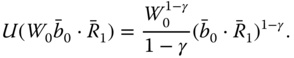
Figure 9.6 plots normalized utility functions with different risk aversion parameters. Panel (a) shows power utility functions (9.28) and panel (b) shows exponential utility functions (9.29). The normalized utility functions are defined by

The normalization is such that ![]() and
and ![]() . Note that the ordering of the distributions according to the expected utility is not affected by linear transformations
. Note that the ordering of the distributions according to the expected utility is not affected by linear transformations ![]() ,
, ![]() ,
, ![]() , because
, because
Figure 9.6 shows that larger values of ![]() or
or ![]() are used when one is more risk averse, because the curvature of the utility functions increases when
are used when one is more risk averse, because the curvature of the utility functions increases when ![]() or
or ![]() are increased.
are increased.

Figure 9.6 Utility functions. (a) Power utility functions (9.28) for risk aversion values  ,
,  , and
, and  ; (b) exponential utility functions (9.29) for risk aversion values
  ,
,  , and
, and  .
.
Figure 9.7 shows contour plots of functions ![]() , where
, where ![]() follows distribution
follows distribution ![]() , where
, where ![]() , where
, where ![]() ,
, ![]() . In panel (a) the utility function is logarithmic
. In panel (a) the utility function is logarithmic ![]() and in panel (b)
and in panel (b) ![]() with
with ![]() .8 The expected utility is maximized when the mean is high and the standard deviation is low, which happens in the upper left corner. We see that for the logarithmic utility the expected utility is determined by the expectation, but increasing the risk aversion to
.8 The expected utility is maximized when the mean is high and the standard deviation is low, which happens in the upper left corner. We see that for the logarithmic utility the expected utility is determined by the expectation, but increasing the risk aversion to ![]() makes the expected utility sensitive both to mean and to standard deviation. When risk aversion is increased more, then the expected utility becomes sensitive only to standard deviation.
makes the expected utility sensitive both to mean and to standard deviation. When risk aversion is increased more, then the expected utility becomes sensitive only to standard deviation.

Figure 9.7 Expected utility as a function of mean and standard deviation. We show contour plots of functions  , where
  follows a normal distribution
  . (a)
. (a)  ; (b)
; (b)  with
with  .
.
9.2.2.3 Taylor Expansion of the Utility
A Taylor expansion of a utility function can be used to gain insight into the differences between the use of the mean–variance criterion and the use of the expected utility, because the use of the mean–variance criterion is approximately equal to the use of the second-order Taylor expansion to approximate the utility function. Also, we can use a Taylor expansion to replace the expected utility with a series containing higher than the second-order moment, which leads to a useful tool in portfolio selection.
We restrict ourselves to the fourth-order Taylor expansion, because the extension to higher order expansions is obvious. For a utility function ![]() that has fourth-order continuous derivatives we have the approximation
that has fourth-order continuous derivatives we have the approximation
where ![]() . This approximation holds for a power utility function
. This approximation holds for a power utility function ![]() , when
, when ![]() and
and ![]() . We can write
. We can write
where ![]() is the risk-free rate and
is the risk-free rate and
is the vector of the excess gross returns. We can choose also ![]() , so that
, so that ![]() is the net return instead of the excess return. When we take
is the net return instead of the excess return. When we take ![]() and
and ![]() , then we obtain the approximation
, then we obtain the approximation
where ![]() ,
, ![]() ,
, ![]() ,
, ![]() , and
, and ![]() .9 As a special case, when
.9 As a special case, when ![]() , then the fourth-order Taylor expansion leads to the approximation
, then the fourth-order Taylor expansion leads to the approximation
Figure 9.8 shows the first four Taylor approximations to the logarithmic utility. The black curve shows log-utility ![]() , the blue curve shows the linear function
, the blue curve shows the linear function ![]() , the red curve shows the quadratic function
, the red curve shows the quadratic function ![]() , the green curve shows the third-order polynomial
, the green curve shows the third-order polynomial ![]() , and the yellow curve shows the fourth-order polynomial
, and the yellow curve shows the fourth-order polynomial ![]() . The approximations are accurate when the gross return is close to one. A gross return close to one means that the asset price has not changed much. However, when the gross return is close to zero or much larger than one, then even the fourth-order approximation is not accurate. Thus, using the logarithmic utility in portfolio selection leads to taking large fluctuations into account, and in particular, the logarithmic utility is better than any finite approximation when we consider portfolios with extreme tail risk: the logarithmic utility approaches
. The approximations are accurate when the gross return is close to one. A gross return close to one means that the asset price has not changed much. However, when the gross return is close to zero or much larger than one, then even the fourth-order approximation is not accurate. Thus, using the logarithmic utility in portfolio selection leads to taking large fluctuations into account, and in particular, the logarithmic utility is better than any finite approximation when we consider portfolios with extreme tail risk: the logarithmic utility approaches ![]() when the gross return approaches zero.
when the gross return approaches zero.

Figure 9.8 Approximation of logarithmic utility. The black curve shows log-utility  , the blue curve shows the linear approximation, the red curve shows the quadratic approximation, the green curve shows the third-order approximation, and the yellow curve shows the fourth-order approximation.
9.2.2.4 Risk Aversion
We can classify utility functions using measures of risk aversion.
CARA Utility Functions
The coefficient of absolute risk aversion of utility function ![]() at point
at point ![]() is defined as
is defined as

Utility functions with constant absolute risk aversion are called CARA utility functions. For example, the exponential utility functions, defined in (9.29), are CARA utility functions and have the coefficient of absolute risk aversion ![]() , whereas the power utility functions, defined in (9.28), are not CARA utility functions because they have the coefficient of absolute risk aversion
, whereas the power utility functions, defined in (9.28), are not CARA utility functions because they have the coefficient of absolute risk aversion ![]() . When an investor whose wealth is 100 is willing to risk 50, and after reaching wealth 1000, is still willing to risk 50, then the investor has constant absolute risk aversion. Most investors have decreasing absolute risk aversion (so that after reaching wealth 1000, the investor is willing to risk more than 50).
. When an investor whose wealth is 100 is willing to risk 50, and after reaching wealth 1000, is still willing to risk 50, then the investor has constant absolute risk aversion. Most investors have decreasing absolute risk aversion (so that after reaching wealth 1000, the investor is willing to risk more than 50).
CRRA Utility Functions
The coefficient of relative risk aversion of utility function ![]() at point
at point ![]() is defined as
is defined as

Utility functions with constant relative risk aversion are called CRRA utility functions. For example, the power utility functions are CRRA utility functions and have the coefficient of relative risk aversion ![]() , whereas the exponential utility functions are not CRRA utility functions because they have the coefficient of relative risk aversion
, whereas the exponential utility functions are not CRRA utility functions because they have the coefficient of relative risk aversion ![]() . When an investor whose wealth is 100 is willing to risk 50, and after reaching wealth 1000, is willing to risk 500, then the investor has constant relative risk aversion.
. When an investor whose wealth is 100 is willing to risk 50, and after reaching wealth 1000, is willing to risk 500, then the investor has constant relative risk aversion.
Expected Utility and Portfolio Weights
It is helpful to plot a curve that shows estimates of the expected utility for a scale of risk aversion parameters. The expected utility curve is the function
where

and ![]() is the power utility function, defined in (9.28). Since the expected value is unknown, we have to estimate it using a sample average of historical values.
is the power utility function, defined in (9.28). Since the expected value is unknown, we have to estimate it using a sample average of historical values.
In the case of two basis assets, it is helpful to look at functions
for various values of ![]() , where
, where ![]() and
and ![]() are the gross returns of the two basis assets.
are the gross returns of the two basis assets.
Figure 9.9 considers daily S&P 500 and Nasdaq-100 data, described in Section 2.4.2. Panel (a) shows functions (9.32) for S&P 500 (black) and Nasdaq-100 (red). We see that Nasdaq-100 is better for a risky investor but S&P 500 is better for a risk averse investor. Panel (b) shows functions (9.33) for ![]() (blue) and
(blue) and ![]() (green). Here
(green). Here ![]() is the return of S&P 500 and
is the return of S&P 500 and ![]() is the return of Nasdaq-100. The optimal value of weight
is the return of Nasdaq-100. The optimal value of weight ![]() is indicated by vertical lines. We see that when risk aversion
is indicated by vertical lines. We see that when risk aversion ![]() increases, then the weight
increases, then the weight ![]() of Nasdaq-100 decreases.
of Nasdaq-100 decreases.

Figure 9.9 Portfolio selection: S&P 500 and Nasdaq-100. (a) Functions (9.32) for S&P 500 (black) and Nasdaq-100 (red); (b) functions (9.33) for  (blue) and
  (green).
Figure 9.10 considers monthly S&P 500 data, described in Section 2.4.3. Panel (a) shows functions
where ![]() is the gross return of S&P 500. Thus,
is the gross return of S&P 500. Thus, ![]() is the gross return of a portfolio whose components are the risk-free rate with gross return one and the S&P 500. We show cases
is the gross return of a portfolio whose components are the risk-free rate with gross return one and the S&P 500. We show cases ![]() (black),
(black), ![]() (red),
(red), ![]() (blue), and
(blue), and ![]() (green). Panel (b) shows functions
(green). Panel (b) shows functions
for ![]() (purple) and
(purple) and ![]() (dark green). The optimal value of weight
(dark green). The optimal value of weight ![]() is indicated by vertical lines.
is indicated by vertical lines.

Figure 9.10 Portfolio selection: Risk-free rate and S&P 500. (a) Functions (9.34) for  (black),
  (red),
  (blue), and
  (green); (b) functions (9.35) for
  (purple) and
  (dark green).
9.2.3 Stochastic Dominance
Sometimes a return distribution stochastically dominates another return distribution, so that it is preferred regardless of the chosen utility function. However, stochastic dominance occurs rarely in practice.
The distribution of ![]() stochastically dominates the distribution of
stochastically dominates the distribution of ![]() , if
, if
for all ![]() , where
, where ![]() and
and ![]() are the distribution functions. Inequality (9.36) is equivalent to
are the distribution functions. Inequality (9.36) is equivalent to
for all ![]() .
.
Stochastic dominance is also called first-order stochastic dominance to distinguish it from second-order stochastic dominance. The distribution of ![]() second-order dominates stochastically the distribution of
second-order dominates stochastically the distribution of ![]() , if
, if

for all ![]() .
.
Figure 9.11 shows an example of first-order stochastic dominance. Panel (a) shows the densities of two distributions, and the distribution of the black density stochastically dominates the distribution of the red density. The densities have the same shape but the black density is located to the right of the red density. Panel (b) shows the distribution functions.

Figure 9.11 First-order stochastic dominance. The black distribution dominates the red distribution. (a) Density functions; (b) distribution functions.
Figure 3.8(b) shows two empirical distribution functions, which are such that neither of the distribution functions dominates the other.
Figure 9.12 shows an example of second-order stochastic dominance. The distribution of the black density dominates the distribution of the red density. Panel (a) shows the densities of the two distributions, panel (b) shows the distribution functions, and panel (c) shows the functions ![]() ,
, ![]() , where
, where ![]() and
and ![]() are the distribution functions. The black and the red densities have the same location, but the red distribution has a larger variance than the black distribution.
are the distribution functions. The black and the red densities have the same location, but the red distribution has a larger variance than the black distribution.

Figure 9.12 Second-order stochastic dominance. The black distribution dominates the red distribution. (a) Density functions; (b) distribution functions; (c) functions  ,
,  , where
  and
and  are the distribution functions.
When a return distribution second-order dominates stochastically another return distribution, then it is preferred, regardless of risk aversion. In fact, it holds that the distribution of ![]() second-order dominates the distribution of
second-order dominates the distribution of ![]() if and only if
if and only if
for every increasing and concave utility function ![]() , which is two times continuously differentiable. First-order stochastic dominance occurs if and only if the dominant distribution has a higher expected utility for all increasing and continuously differentiable utility functions.
, which is two times continuously differentiable. First-order stochastic dominance occurs if and only if the dominant distribution has a higher expected utility for all increasing and continuously differentiable utility functions.
9.3 Multiperiod Portfolio Selection
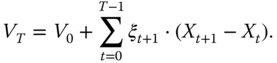
In the multiperiod model the wealth of the portfolio is obtained from (9.10) as

where ![]() is the initial wealth at time 0,
is the initial wealth at time 0, ![]() is the vector of the portfolio weights, and
is the vector of the portfolio weights, and ![]() is the vector of gross returns of the
is the vector of gross returns of the ![]() portfolio components. We write
portfolio components. We write
where ![]() ,
, ![]() . The portfolio weights satisfy
. The portfolio weights satisfy

Now ![]() is the one period gross return. We can write
is the one period gross return. We can write
![]() . In this way we do not have to worry about the restriction (9.39).
. In this way we do not have to worry about the restriction (9.39).
The wealth of the portfolio is obtained in additive form from (9.13) as
where

Here

The vector ![]() gives the numbers of risky assets in the portfolio. Vector
gives the numbers of risky assets in the portfolio. Vector ![]() is unrestricted. Note that the time indexing is such that
is unrestricted. Note that the time indexing is such that ![]() and
and ![]() both describe the portfolio for the period
both describe the portfolio for the period ![]() . Note that we have assumed in (9.41) that
. Note that we have assumed in (9.41) that ![]() almost surely. This holds when
almost surely. This holds when ![]() is a risk-free investment.
is a risk-free investment.
The multiplicative way of writing the wealth presupposes a positive wealth, whereas the additive way of writing the wealth allows for a nonpositive wealth. The multiplicative way of writing the wealth is convenient for the power utility functions, whereas the additive way of writing the wealth is convenient for the exponential utility functions, because factoring the wealth as a product makes the writing of the backward induction convenient.
At time ![]() we want to find the portfolio vector
we want to find the portfolio vector ![]() or
or ![]() so that
so that
is maximized, where the rebalancing of the portfolio will be made at times ![]() . The maximization of (9.42) is over the sequence of weights
. The maximization of (9.42) is over the sequence of weights ![]() or over the sequence of numbers
or over the sequence of numbers ![]() , although at time
, although at time ![]() we need to choose only
we need to choose only ![]() or
or ![]() .
.
We can summarize the results in the following way:
- 1. For the logarithmic utility function the multiperiod portfolio selection reduces to the one-period portfolio selection.
- 2. For the power utility functions (which include the logarithmic utility) and for the exponential utility functions the optimal portfolio vector does not depend on the initial wealth.
The power utility functions need a positive wealth as the argument, and they can be applied when the wealth process is written in the product form. The exponential utility functions can take a negative wealth as the argument, and they lead to tractable dynamic programming when the wealth process is written additively.
We describe first the one-period optimization in Section 9.3.1, and then the multiperiod optimization in Section 9.3.2. The understanding of the multiperiod optimization is easier when it is contrasted with the single period optimization. We describe first the case of the logarithmic utility function. After that we describe the solution for the power utility functions. Third, we describe the case of the exponential utility functions. In the multiperiod model we give also the formulas for arbitrary utility functions.
9.3.1 One-Period Optimization
We want to maximize at time 0 the expected utility of the wealth at time 1:
We discuss the cases where ![]() is the logarithmic utility function, a power utility function, and an exponential utility function.
is the logarithmic utility function, a power utility function, and an exponential utility function.
9.3.1.1 The Logarithmic Utility Function
The logarithmic utility function is ![]() . We have
. We have
Thus, we need to maximize
over ![]() , under restriction
, under restriction ![]() . Thus, the optimal
. Thus, the optimal ![]() does not depend on the initial wealth
does not depend on the initial wealth ![]() .
.
The maximization can be done unrestricted when we apply (9.40), so that we need to maximize
over ![]() .
.
9.3.1.2 The Power Utility Functions
The power utility functions are ![]() for
for ![]() , where
, where ![]() ,
, ![]() . We have
. We have
Thus, we need to maximize
over ![]() , under restriction
, under restriction ![]() . Thus, the optimal
. Thus, the optimal ![]() does not depend on the initial wealth
does not depend on the initial wealth ![]() .
.
The maximization can be done unrestricted when we apply (9.40), so that we need to maximize
over ![]() .
.
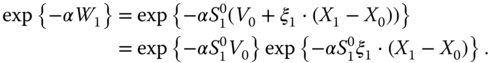
9.3.1.3 The Exponential Utility Functions
The exponential utility functions are ![]() for
for ![]() , where
, where ![]() . The maximization of
. The maximization of ![]() is equivalent to the minimization of
is equivalent to the minimization of
We apply the additive form in (9.41) to obtain
Thus, we need to minimize
over ![]() . This is unrestricted minimization. The optimal
. This is unrestricted minimization. The optimal ![]() does not depend on the initial wealth
does not depend on the initial wealth ![]() .
.
9.3.2 The Multiperiod Optimization
We want to maximize at time 0 the expected utility of the wealth at time ![]() :
:
We discuss the cases where ![]() is the logarithmic utility function, a power utility function, an exponential utility function, and a general utility function.
is the logarithmic utility function, a power utility function, an exponential utility function, and a general utility function.
9.3.2.1 The Logarithmic Utility Function
For the logarithmic utility ![]() we have from (9.38) that
we have from (9.38) that

where
We want to find portfolio vector ![]() maximizing
maximizing
under restriction ![]() . We see that for the logarithmic utility the optimal portfolio vector at time
. We see that for the logarithmic utility the optimal portfolio vector at time ![]() is the maximizer over
is the maximizer over ![]() of the single period expected logarithmic return
of the single period expected logarithmic return
when the maximization is done under restriction ![]() . In particular, the initial wealth
. In particular, the initial wealth ![]() does not affect the solution.
does not affect the solution.
We can use (9.40) to note that the maximization can be done without the restriction: we need to maximize
over ![]() .
.
We have shown that in the case of the logarithmic utility the multiperiod optimization reduces to the single period optimization, since ![]() can be found by ignoring the time points
can be found by ignoring the time points ![]() .
.
9.3.2.2 The Power Utility Functions
Let ![]() be the power utility function
be the power utility function

where ![]() is the risk aversion parameter. For
is the risk aversion parameter. For ![]() we define
we define ![]() . For
. For ![]() we get from (9.38) that
we get from (9.38) that
Thus, for ![]() we need to maximize
we need to maximize

under restrictions
where
Thus, the optimal portfolio vector ![]() does not depend on the initial wealth
does not depend on the initial wealth ![]() .
.
Using (9.40) we see that we can maximize

over ![]() ,
, ![]() .
.
The Case 
Let us consider the maximization of (9.44) for the case ![]() . We present first the case
. We present first the case ![]() because the structure of the argument is visible already in the two period case but this case is notationally more transparent than the general case
because the structure of the argument is visible already in the two period case but this case is notationally more transparent than the general case ![]() . Define function
. Define function
where
The optimal portfolio vector at time ![]() is the maximizer of function
is the maximizer of function ![]() : Our purpose is to find
: Our purpose is to find
We can write, using the law of the iterated expectations,
Thus,

Comparing to (9.43) we see the difference between the one- and two-period portfolio selections: In the two-period case, we have the additional multiplier ![]() .
.
We can use (9.40) to note that the maximization can be done without the restrictions. Write
where ![]() and
and ![]() are unrestricted.
are unrestricted.
The Case 
Let us consider the maximization of (9.44). Define

where , ![]() ,
,
Here ![]() means the
means the ![]() fold product
fold product ![]() . The optimal portfolio vector a time
. The optimal portfolio vector a time ![]() is the maximizer of function
is the maximizer of function ![]() : Our purpose is to find
: Our purpose is to find
We give a recursive formula for ![]() .
.
- 1. Denote

- and let
 be the maximizer of
  over
over  .
. - 2. For
 , define

- and let
 be the maximizer of
  over
over  .
.
We can use (9.40) to note that the maximization can be done without the restrictions: we can define the functions to be maximized as
and
![]() . The maximization is done over
. The maximization is done over ![]() in the one before the previous function, and over
in the one before the previous function, and over ![]() in the previous function.
in the previous function.
9.3.2.3 The Exponential Utility Functions
Let ![]() be the exponential utility function
be the exponential utility function
where ![]() is the risk aversion parameter. Maximizing
is the risk aversion parameter. Maximizing ![]() is equivalent to minimizing
is equivalent to minimizing ![]() . We get from (9.41) that
. We get from (9.41) that

Thus, we need to minimize

over ![]() , where
, where
Thus, the optimal portfolio vector ![]() does not depend on the initial wealth
does not depend on the initial wealth ![]() .
.
Define

The optimal portfolio vector a time ![]() is the minimizer of function
is the minimizer of function ![]() : Our purpose is to find
: Our purpose is to find
We give a recursive formula for ![]() .
.
- 1. Denote

- and let
 be the minimizer of
  over
over  .
. - 2. For
 , define

- and let
 be the minimizer of
  over
over  .
.
9.3.2.4 General Utility Functions
When the utility function is not the logarithmic function, of a power form, or of an exponential form, then the maximizer of the expected wealth can depend on the initial wealth. Also, for the general utility functions we do not obtain such factorization as for the logarithmic and power utility functions (when the product form is used) or such factorization as for the exponential utility functions (when the additive form is used). However, we can obtain recursive formulas for the maximization of the expected wealth.
The Product Form
The optimal portfolio vector at time ![]() is defined as the maximizer of the expected utility
is defined as the maximizer of the expected utility ![]() . Thus, the optimal portfolio vector maximizes function
. Thus, the optimal portfolio vector maximizes function ![]() , defined as
, defined as

where
We can define the optimal portfolio vector recursively as follows:
- 1. Define

- and let
 be the maximizer of
  over
over  .
. - 2. For
 , define

- where

- Let
 be the maximizer of
  over
over  .
.
This gives a recursive definition of ![]() .10
.10
The Additive Form
The optimal portfolio vector at time ![]() is defined as the maximizer of the expected utility
is defined as the maximizer of the expected utility ![]() . Thus, the optimal portfolio vector maximizes function
. Thus, the optimal portfolio vector maximizes function ![]() , defined as
, defined as

We can define the optimal portfolio vector recursively as follows:
- 1. Define

- and let
 be the maximizer of
  over
over  .
. - 2. For
 , define

- where

- Let
 be the maximizer of
  over
over  .
.
This gives a recursive definition of ![]() .
.

Then,


where ![]() .
.
We can write, using the law of the iterated expectations,
Thus, in the two-period case,
