
Chapter 13
Principles of Asset Pricing
Asset pricing can be studied in two different settings: absolute pricing and relative pricing. Absolute pricing tries to explain the prices in terms of fundamental macroeconomic variables, applying utility functions and preferences. Relative pricing tries to explain the prices of a group of assets given the prices of a more fundamental group of assets.
We concentrate on relative pricing. Derivatives are assets whose payoffs are defined in terms of the payoffs of some basis assets. For example, an European call option gives the right to buy the underlying asset at the given expiration time ![]() at the given strike price
at the given strike price ![]() . Thus, the payoff of the call option at time
. Thus, the payoff of the call option at time ![]() is equal to
is equal to
where ![]() is the value of the underlying asset. We want to find a “fair price”
is the value of the underlying asset. We want to find a “fair price” ![]() for the call option, when
for the call option, when ![]() is a previous time.
is a previous time.
Derivatives are traded in exchanges just like stocks, and the price of a derivative is determined in an exchange by supply and demand. It can be argued that the pricing of the market is typically efficient. However, it is of interest to try to find fair prices by statistical and probabilistic methods at least for the following two reasons. (1) Sometimes options are bought and sold over the counter and not in exchanges. In this case, there is no information provided by the markets. (2) It is possible that the market prices are irrational. This can certainly happen in illiquid markets. In this case, a market participant can profit from the knowledge of scientific methods of pricing.
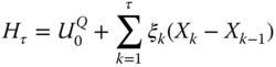
Besides pricing of options, it is of equal importance to hedge options. In fact, our main emphasis will be on the pricing by quadratic hedging. In this approach, the price of an option will be the initial investment of a trading strategy, which minimizes the quadratic error
where ![]() is the wealth obtained by the hedging strategy, and
is the wealth obtained by the hedging strategy, and ![]() is the value of the derivative at the expiration. This approach will be developed more in detail in Chapter 16.
is the value of the derivative at the expiration. This approach will be developed more in detail in Chapter 16.
Section 13.1 studies general principles of pricing heuristically, discussing such concepts as absolute and relative pricing, arbitrage, the law of one price, and completeness of models. In addition, we introduce the idea of quadratic hedging.
Section 13.2 presents basics of mathematical asset pricing in discrete time. We describe the first and the second fundamental theorems of asset pricing (Theorems 13.1 and 13.3). The first fundamental theorem says that a market is arbitrage-free if and only if there exists an equivalent martingale measure. The second fundamental theorem says that every derivative can be replicated if and only if the martingale measure is unique. If every derivative can be replicated, then it is said that the market is complete. Theorem 13.2 states that the arbitrage-free prices of European options are expectations with respect to an equivalent martingale measure.
We give a proof of the first fundamental theorem of asset pricing. The proof is constructive: we construct an equivalent martingale measure for an arbitrage-free market. The most proofs of the first fundamental theorem of asset pricing found in the literature are not constructive, but apply abstract functional analysis. However, the construction of suitable equivalent martingale measures is useful for practical applications, because these measures lead to the collections of arbitrage-free prices. We do not give a proof of the second fundamental theorem of asset pricing. This is due to the fact that the general theory of complete markets seems to be less relevant from the practical point of view than the theory of incomplete markets, although the Black–Scholes model is useful in applications. Chapter 14 describes the theory of Black–Scholes pricing and Chapter 15 is devoted to incomplete models.
Section 13.3 discusses methods for the comparison of different pricing and hedging methods. The main method for the comparison is to use historical simulation to generate trajectories of prices, hedge the derivative through the trajectories, and then compute the sample mean of the squared hedging errors.
13.1 Introduction to Asset Pricing
Section 13.1.1 discusses absolute pricing with the help of coin tossing games. These examples show that utility functions can be useful in determining reasonable prices. Section 13.1.2 discusses how the principle of excluding arbitrage and the law of one price can be applied in relative pricing. The one period binary model is introduced. This model will be used to derive the Black–Scholes prices in Chapter 14. Section 13.1.3 discusses relative pricing in cases where arbitrage cannot be applied. The one period ternary model is an example of such case. In these cases, a fair price can be defined by minimizing the mean squared hedging error, for example.
13.1.1 Absolute Pricing
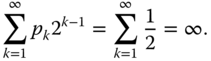
Let us consider a coin tossing game where a participant receives 1 € when heads occur and 0 € when tails occurs. The probability of getting heads is 1/2 and the probability of obtaining tails is 1/2. What is the fair price to participate in this game? It can be argued that the fair price is the expected gain:
The fairness of the price can be justified by the law of large numbers. The law of large numbers implies that the gain from repeated independent repetitions of the game with price 0.5 € converges to zero with probability 1. A larger price than 0.5 € would give an almost sure profit to the organizer of the game in the long run and a smaller price than 0.5 € would give an almost sure profit to the player of the game in the long run.
It does not seem as clear what the price should be if we change the game so that a participant receives 1 million € when heads occur and 0 € when tails occur. Only few people would be willing to invest half a million € in order to participate in this game. The law of large numbers cannot be applied to justify a price because the probability of a bankruptcy is quite large when a player repeats the game.1
It can be argued that the price of the game should be equal to the expected utility: Let ![]() be the random variable with
be the random variable with ![]() and
and ![]() , where
, where ![]() million €. Then the expected utility is
million €. Then the expected utility is ![]() , where
, where ![]() is a utility function.
is a utility function.
The St. Petersburg paradox can be used to suggest that a utility function should be used. In the St. Petersburg paradox, the banker flips the coin until the heads come out the first time. The player receives ![]() coins when there are
coins when there are ![]() tosses of the coin (1 coin if the heads come out in the first toss, 2 coins if the heads come out in the second toss, 4 coins if the heads come out in the third toss, and so on). What is the fair entrance fee to the game? We can calculate the expected gain. The probability that there are
tosses of the coin (1 coin if the heads come out in the first toss, 2 coins if the heads come out in the second toss, 4 coins if the heads come out in the third toss, and so on). What is the fair entrance fee to the game? We can calculate the expected gain. The probability that there are ![]() tosses is
tosses is ![]() . Thus the expected payoff is
. Thus the expected payoff is
Thus, it would seem that the entrance fee could be arbitrarily high. However, applying common sense, it does not seem reasonable to pay a high entrance fee. The paradox can be solved by using a utility function to measure the utility of the wealth. For example, the logarithmic utility function ![]() gives the expected utility of the game
gives the expected utility of the game

which would give the price of two coins for the game.2
The St Petersburg paradox suggests that we could use the expected utility instead of the expected monetary payoff to determine fair prices. Utility maximization will be discussed in Section 15.2.5, as a method for derivative pricing, but otherwise we do not study further this approach.
13.1.2 Relative Pricing Using Arbitrage
Sometimes relative pricing can be done solely by applying the principle of excluding arbitrage. We illustrate this type of relative pricing using a coin tossing example.3 After that, arbitrage and the law of one price are discussed more generally.
13.1.2.1 Pricing in a One Period Binary Model
Let us consider two games related to the same tossing of a coin. The first game is such that the player receives ![]() € when heads occur and
€ when heads occur and ![]() € when tails occurs, where
€ when tails occurs, where ![]() . The participation to this game can be compared to buying a stock. We denote with
. The participation to this game can be compared to buying a stock. We denote with ![]() the random variable with
the random variable with ![]() and
and ![]() .
.
The second game is such that the player receives 1 € when heads occur and 0 € when tails occurs. The participation to this game can be compared to buying a derivative. Indeed, the second game can be considered as a derivative because the payoff in the second game is random variable ![]() for
for ![]() , where
, where ![]() and
and ![]() . Random variable
. Random variable ![]() has the distribution
has the distribution ![]() and
and ![]() . The third asset is a bond with value
. The third asset is a bond with value ![]() . The price of bond is 1 and the price of stock is denoted with
. The price of bond is 1 and the price of stock is denoted with ![]() . We want to find the price of the derivative.
. We want to find the price of the derivative.
The derivative can be replicated with the bond and the stock: Consider the portfolio with ![]() bonds and
bonds and ![]() stocks. We choose
stocks. We choose
The replicating portfolio is ![]() . Indeed, we have that
. Indeed, we have that ![]() , because
, because

By the law of one price, to exclude the possibility of arbitrage, the price of the derivative has to be equal to the price of the portfolio:4
The price of the portfolio is
Thus, the price of the derivative is
The price of the derivative is in general not equal to 0.5. If ![]() , then the price of the derivative is
, then the price of the derivative is ![]() . If
. If ![]() , then the price of the derivative satisfies
, then the price of the derivative satisfies ![]() .5
.5
We have given the price of the derivative in (13.1) in terms of the price of the stock. This is an example of relative pricing: a price of an asset is expressed in terms of the prices of another asset.
13.1.2.2 Arbitrage
Arbitrage is both a term of everyday language and a technical term used in mathematical finance.
Arbitrage is used in everyday language to denote a financial operation where one obtains a profit with probability one by a simultaneous selling and buying of assets. We give two examples of this type of arbitrage.
- 1. The stock of Daimler is listed both in Frankfurt and Stuttgart stock exchanges. If the stock can be bought in Frankfurt with the price of 10 € and sold in Stuttgart with the price of 11 €, we obtain a risk free profit of 1 € (minus the transaction costs).
- 2. Suppose the price of a stock is 10 € and a call option with strike price
 € with the expiration time in 1 week can be bought with the price of 1 €. Then, we can sell the stock short and buy the call option. The profit of the operation will be
  € (buying the call costs 1 €, selling the stock short gives 10 €, and exercising the option costs 8 €).
In general, we have a lower bound
 for the price of a call option, where
  is the price of the stock at the time of buying the option, and
  is the strike price. See (14.9) for a more precise lower bound.
In mathematical finance, an arbitrage is a financial operation whose payoff is always nonnegative and sometimes positive, that is, the probability of a nonnegative payoff is one and the probability of a positive payoff is greater than zero. More formally, arbitrage portfolio ![]() is such that its value at time
is such that its value at time ![]() satisfies
satisfies ![]() but its value
but its value ![]() at a later time
at a later time ![]() satisfies
satisfies ![]() and
and ![]() . A reasonable system of prices should be such that arbitrage is excluded, so that there does not exist an arbitrage portfolio.
. A reasonable system of prices should be such that arbitrage is excluded, so that there does not exist an arbitrage portfolio.
The absence of arbitrage implies the law of one price.
13.1.2.3 The Law of One Price and the Monotonicity Theorem
The law of one price states that if two financial assets have the same payoffs then they have the same price: If two portfolios satisfy
then their prices are equal at a previous time ![]() :
:
The absence of arbitrage implies that the law of one price holds. Indeed, consider the case where the law of one price does not hold. Then we have two assets with different prices at time ![]() , say
, say ![]() , and the prices of the assets are the same with probability 1 at a later time
, and the prices of the assets are the same with probability 1 at a later time ![]() :
: ![]() . Then we can by the cheaper asset at time
. Then we can by the cheaper asset at time ![]() and sell the more expensive asset at time
and sell the more expensive asset at time ![]() to obtain the amount
to obtain the amount ![]() . This amount can be put into a bank account. At time
. This amount can be put into a bank account. At time ![]() the two assets have the same price, and thus we have locked the profit of time
the two assets have the same price, and thus we have locked the profit of time ![]() . We have shown that there exists an arbitrage opportunity. Thus we have shown that the absence of arbitrage implies that the law of one price holds.
. We have shown that there exists an arbitrage opportunity. Thus we have shown that the absence of arbitrage implies that the law of one price holds.
The monotonicity theorem states that if two financial assets satisfy
then their prices satisfy
at time ![]() . Furthermore, if
. Furthermore, if ![]() , then their prices satisfy
, then their prices satisfy ![]() at time
at time ![]() . This formulation of the monotonicity theorem is similar to the formulation of Blyth (2014, p. 48).
. This formulation of the monotonicity theorem is similar to the formulation of Blyth (2014, p. 48).
The law of one price implies the linearity of the pricing function. Let
be a portfolio, and let ![]() be the prices of the basis assets at time
be the prices of the basis assets at time ![]() . Then the price of the portfolio at time
. Then the price of the portfolio at time ![]() is
is
13.1.2.4 Pricing using The Law of One Price
The law of one price can be used to price linear assets by replication.6 Furthermore, the law of one price can be used to price all assets in complete markets. By a market we mean a collections of tradable assets together with assumptions about the probability distributions of the asset values. A complete market is such that any possible payoff can be obtained by a portfolio of assets. That is, assume that the market has tradable assets ![]() . Assume that an arbitrary payoff
. Assume that an arbitrary payoff ![]() can be obtained, so that
can be obtained, so that ![]() . The law of one price implies that price of this payoff is
. The law of one price implies that price of this payoff is
where we applied the linearity in (13.2).
Futures are linear derivatives, and thus the law of one price can be used to price futures; see Section 14.1. Futures can be priced by the law of one price because futures can be defined as a portfolio of the underlying asset and a bond: the payoff of a futures contract is a linear combination of the payoffs of the underlying asset and a bond.
The payoff of an option is not a linear function of the payoff of the underlying. Thus options cannot be priced as easily as futures. The law of one price can be used to price options in the Black–Scholes model, because the Black–Scholes model is a complete model for the markets, so that all derivatives can be replicated (linearly).
The law of one price can be used to derive the put-call parity, which says that the prices of two options satisfy an equation. The law of one price can also be used to give bounds to option prices without assuming the Black–Scholes model, or any other market model. See Section 14.1.2 for the derivation of the put-call parity.
13.1.3 Relative Pricing Using Statistical Arbitrage
We have derived the price of the derivative in (13.1) using the replication of the derivative with a stock and a bond. The exact replication is possible only under special circumstances. It suffices to move from the binary model to a ternary model to make exact replication impossible, so that only approximate replication is possible. We use the term “statistical arbitrage” to mean quadratic hedging (variance optimal hedging), quantile hedging, and other similar methods for approximate replication.
13.1.3.1 Pricing in a One Period Ternary Model
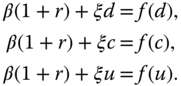
Let us have two games related to the same tossing of a dice. The first game is such that the player receives ![]() € when the dice shows 1 or 2,
€ when the dice shows 1 or 2, ![]() € when the dice shows 3 or 4, and
€ when the dice shows 3 or 4, and ![]() € when the dice shows 5 or 6, where
€ when the dice shows 5 or 6, where ![]() . The participation to this game is an analogy to buying a stock and we denote with
. The participation to this game is an analogy to buying a stock and we denote with ![]() the random variable with
the random variable with ![]() .
.
The second game is such that the player receives 0 € when the dice shows 1, 2, 3, or 4 and 1 € when the dice shows 5 or 6. The participation to this game is an analogy to buying a derivative and we denote with ![]() the random variable
the random variable ![]() , where
, where ![]() is defined by
is defined by ![]() when
when ![]() and
and ![]() when
when ![]() . Now
. Now ![]() and
and ![]() . The third asset is a bond with value
. The third asset is a bond with value ![]() . The price of the bond is 1 and the price of the stock is denoted with
. The price of the bond is 1 and the price of the stock is denoted with ![]() . We want to find the price
. We want to find the price ![]() of the derivative.
of the derivative.
The derivative cannot be replicated with the bond and the stock: Consider the portfolio with ![]() bonds and
bonds and ![]() stocks. The portfolio is
stocks. The portfolio is ![]() . We have
. We have ![]() when
when ![]() and
and ![]() satisfy
satisfy

We can typically not find such ![]() and
and ![]() because, in general, two parameters cannot satisfy three equations simultaneously. To obtain an approximate replication we could choose
because, in general, two parameters cannot satisfy three equations simultaneously. To obtain an approximate replication we could choose ![]() and
and ![]() so that
so that ![]() is minimized. We have that
is minimized. We have that

Since the probabilities are all equal to ![]() , we get the least squares solution for
, we get the least squares solution for ![]() :
:
where

The solution is

We set the price of the derivative to be equal to the price of the approximately replicating portfolio:
If ![]() , then
, then ![]() .
.
13.1.3.2 Statistical Arbitrage and the Law of Approximate Price
Statistical arbitrage is a financial operation where a profit is obtained with a high probability. The principle of excluding statistical arbitrage is a pricing principle, which can be used when the principle of excluding arbitrage does not apply. However, the concept of statistical arbitrage can be defined in many ways. Let us compare the principle of excluding arbitrage to the idea of excluding statistical arbitrage.
- 1. Excluding arbitrage. The value of a derivative is
 at time
  . Let us have another asset whose value is
  at time
  . Assume that the values are equal with probability 1:
  . Then it should hold that the value of the derivative and the other asset are equal at all previous times:
  for all previous times
  . Otherwise, there would be an arbitrage opportunity: sell the more expensive instrument and buy the cheaper instrument to obtain a risk free profit at time
  .
. - 2. Excluding statistical arbitrage. The value of a derivative is
 at time
  . Let us have an other asset whose value is
  at time
  . If the random variables
  and
and  are “close,” then the prices
  and
and  should be close at all previous times
  . The closeness of random variables can be defined in many ways. For example, we can say that two random variables
  and
and  are close when
  is small. A derivative can be priced with statistical arbitrage if we can construct an asset, which replicates the payoff of the derivative with high probability.
Pricing with statistical arbitrage requires that we define the best approximation ![]() to a random payoff
to a random payoff ![]() . As an example, we can consider a call option written at time
. As an example, we can consider a call option written at time ![]() , with the strike price
, with the strike price ![]() and with the expiration time
and with the expiration time ![]() . The payout of the option at the expiration time is
. The payout of the option at the expiration time is ![]() , where
, where ![]() is the price of the underlying instrument at time
is the price of the underlying instrument at time ![]() . The best constant approximation of random variable
. The best constant approximation of random variable ![]() in the sense of mean squared error is its expectation:7
in the sense of mean squared error is its expectation:7
where the minimization is taken with respect to all real numbers. Thus, expectation ![]() can give a first approximation to the price of
can give a first approximation to the price of ![]() . We can use the underlying asset to provide a better approximation. The best approximation of
. We can use the underlying asset to provide a better approximation. The best approximation of ![]() with a function
with a function ![]() of
of ![]() is the conditional expectation:
is the conditional expectation:
where the minimization is taken with respect to functions ![]() , and function
, and function ![]() takes values
takes values ![]() . Thus, the conditional expectation
. Thus, the conditional expectation ![]() could be a candidate for the fair price. However, the conditional expectation is typically not a tradable asset, and we will make a further restriction to find such function
could be a candidate for the fair price. However, the conditional expectation is typically not a tradable asset, and we will make a further restriction to find such function ![]() , which is tradable, which leads to linear approximations.
, which is tradable, which leads to linear approximations.
13.2 Fundamental Theorems of Asset Pricing
Our intention is to describe the basic mathematical terminology and fundamental theorems of asset pricing in discrete time models. Our presentation follows Shiryaev (1999) and Föllmer and Schied (2002). The mathematics of asset pricing is a fascinating topic with elegant results and we hope that the presentation will inspire readers to study the subject in a greater detail.
The first fundamental theorem of asset pricing says that a market is arbitrage-free if and only if there exists an equivalent martingale measure. Furthermore, these martingale measures define the collection of arbitrage-free prices for a derivative. In a complete model, there is exactly one equivalent martingale measure, but in an incomplete model there are many equivalent martingale measures. Thus, the main problem will be to choose the martingale measure for pricing from a collection of available martingale measures. Our emphasis will be in incomplete models.
13.2.1 Discrete Time Markets
Let ![]() be the time series of prices of a riskless bond (bank account). Let
be the time series of prices of a riskless bond (bank account). Let ![]() be the vector time series of prices of risky assets, where
be the vector time series of prices of risky assets, where ![]() . The price vector that contains both the bond and the risky assets is denoted by
. The price vector that contains both the bond and the risky assets is denoted by
13.2.1.1 Filtered Probability Spaces
The underlying probability space ![]() is accompanied with a filtration of sigma-algebras
is accompanied with a filtration of sigma-algebras ![]() .8 The price process of stocks is adapted with respect to the filtration:
.8 The price process of stocks is adapted with respect to the filtration: ![]() is measurable with respect to
is measurable with respect to ![]() .9 The price process of the bond is predictable with respect to the filtration:
.9 The price process of the bond is predictable with respect to the filtration: ![]() is measurable with respect to
is measurable with respect to ![]() ,
, ![]() , and
, and ![]() is measurable with respect to
is measurable with respect to ![]() . Thus, the value of
. Thus, the value of ![]() is known at time
is known at time ![]() , which makes
, which makes ![]() locally riskless. The prices are assumed to be nonnegative. We assume that10
locally riskless. The prices are assumed to be nonnegative. We assume that10
Thus, ![]() and elements of
and elements of ![]() are constants (with probability 1).
are constants (with probability 1).
13.2.1.2 Trading Strategies
A trading strategy is
The values ![]() and
and ![]() express the quantity of the bond and the
express the quantity of the bond and the ![]() th asset held between
th asset held between ![]() and
and ![]() . The trading strategy is predictable:
. The trading strategy is predictable: ![]() and
and ![]() are measurable with respect to
are measurable with respect to ![]() . This means that
. This means that ![]() and
and ![]() are determined at time
are determined at time ![]() , using the information available at time
, using the information available at time ![]() .
.
13.2.1.3 Examples
Let us give examples of the locally riskless bond ![]() . We can take
. We can take ![]() , where
, where ![]() is a constant, or
is a constant, or ![]() , where
, where ![]() . In addition, we can take
. In addition, we can take ![]() , and
, and

for ![]() , where
, where ![]() is predictable. We can also take
is predictable. We can also take ![]() and
and ![]() , where
, where ![]() is predictable.
is predictable.
Consider the two period binary model as an example of adaptability and predictability. Now ![]() and
and ![]() . The initial stock price is
. The initial stock price is ![]() . The next price is
. The next price is ![]() and the final price is
and the final price is ![]() , where
, where ![]() and
and ![]() are random variables. Random variable
are random variables. Random variable ![]() satisfies
satisfies ![]() and
and ![]() for
for ![]() , where
, where ![]() is a fixed constant. Random variable
is a fixed constant. Random variable ![]() has the same distribution as
has the same distribution as ![]() , and is independent of
, and is independent of ![]() . Choose
. Choose
where ![]() and
and ![]() refer to the upwards and downwards movements of the stock. Set
refer to the upwards and downwards movements of the stock. Set ![]() describes all possible trajectories of the process. Now,
describes all possible trajectories of the process. Now,

Let ![]() . It follows that
. It follows that

In order for the stock prices to be adapted to the filtration we need
We have that

It follows that in order for the stock prices to be adapted to the filtration we need
Let the initial bond price be ![]() . Let the next bond price be
. Let the next bond price be ![]() , where
, where ![]() is a constant. Let the final bond price be
is a constant. Let the final bond price be ![]() , where
, where ![]() . Now bond prices are predictable with respect to the filtration. Bond price at time
. Now bond prices are predictable with respect to the filtration. Bond price at time ![]() depends only on the stock price at time
depends only on the stock price at time ![]() . Thus, the bond price at time
. Thus, the bond price at time ![]() is a random variable which is known at time
is a random variable which is known at time ![]() .
.
13.2.2 Wealth and Value Processes
We define the wealth and value processes. The value process is obtained from the wealth process by dividing with the bond price. After that we derive an expression for the wealth and value processes under the assumption of self-financing.
13.2.2.1 The Wealth and Value Processes
We use the following notation for the inner product:

At time 0 the initial wealth is ![]() and after that,
and after that,
Indeed, the portfolio vector ![]() is chosen at time
is chosen at time ![]() and hold during the period
and hold during the period ![]() .
.
We assume that ![]() for all
for all ![]() and choose the bond as a numéraire. The discounted price process is defined by
and choose the bond as a numéraire. The discounted price process is defined by

We denote
The value process is defined as ![]() and
and

13.2.2.2 The Wealth Process under Self-financing
We assume in most cases that the trading strategy is self-financing. The local quadratic hedging without self-financing in Section 16.2.3 is a case where self-financing is not assumed.
Let us describe trading under the condition of self-financing. At time 0 the initial wealth is ![]() . The wealth is allocated among the available assets: the quantities
. The wealth is allocated among the available assets: the quantities ![]() are chosen so that
are chosen so that
The prices change from ![]() to
to ![]() , and the wealth changes accordingly from
, and the wealth changes accordingly from ![]() to
to ![]() . After that, wealth
. After that, wealth ![]() is allocated among the available assets. We obtain
is allocated among the available assets. We obtain
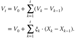
We continue in this way to obtain
The final wealth is
At time ![]() we need not do the reallocation, because it is the last time instance.
we need not do the reallocation, because it is the last time instance.
We have described a process of trading, which is self-financing. We say that a trading strategy ![]() is self-financing if
is self-financing if
When the trading strategy is self-financing, then no external funds are received, and no funds are reserved for consumption.
Under the assumption (13.4) of self-financing, the change of wealth can be written as
for ![]() . Thus, the wealth at time
. Thus, the wealth at time ![]() can be written as11
can be written as11

where ![]() .
.
13.2.2.3 The Value Process Under Self-Financing
Let us assume that the rebalancing is made respecting the condition of self-financing: ![]() is chosen so that the wealth
is chosen so that the wealth ![]() is allocated among the assets. Equation
is allocated among the assets. Equation ![]() sets a linear constraint on the vector
sets a linear constraint on the vector ![]() . It is convenient to write the wealth process so that the quantity
. It is convenient to write the wealth process so that the quantity ![]() of bonds is eliminated, and this can be done using the value process.
of bonds is eliminated, and this can be done using the value process.
The self-financing condition in (13.4) implies that the discounted price process ![]() in (13.3) satisfies
in (13.3) satisfies
Similarly as for the wealth process, it holds that

Under the condition (13.6) of self-financing, an increment of the value process can be written as
where the last equality follows because the first element of ![]() is 1 for all
is 1 for all ![]() . Thus, the value at time
. Thus, the value at time ![]() can be written as
can be written as
Note that the value process is written in terms of the quantity ![]() of stocks. The quantity
of stocks. The quantity ![]() of bonds is obtained from the equations
of bonds is obtained from the equations

which follow from self-financing equations (13.7).
The gains process is defined as

For a self-financing strategy
The gains process is a discrete stochastic integral. The gains process is a transformation of ![]() by means of
by means of ![]() .12
.12
The value process can be used to derive some expressions for the wealth. For example, when ![]() , then13
, then13

13.2.3 Arbitrage and Martingale Measures
An arbitrage opportunity is a self-financing trading strategy ![]() so that its value process satisfies
so that its value process satisfies
This means that with an initial investment of zero it is possible to get a final wealth, which is always nonnegative and sometimes positive.
A martingale is a stochastic process ![]() on a filtered probability space
on a filtered probability space ![]() if14
if14
- 1.
 it is adapted (
 is
is  measurable),
 - 2.
 for
for  ,
, - 3.
 for
for  .
.
A martingale difference satisfies conditions 1 and 2, but condition 3 takes the form ![]() for
for ![]() . Thus, a martingale difference is a martingale if
. Thus, a martingale difference is a martingale if ![]() .
.
A probability measure ![]() on
on ![]() is called a martingale measure, or a risk neutral measure, if the discounted price process
is called a martingale measure, or a risk neutral measure, if the discounted price process ![]() is a
is a ![]() -dimensional martingale. Then,
-dimensional martingale. Then,

for ![]() , and
, and

![]() -almost surely for
-almost surely for ![]() , where
, where ![]() .
.
An equivalent martingale measure is a martingale measure, which is equivalent to the original measure ![]() . Measures
. Measures ![]() and
and ![]() are equivalent, if
are equivalent, if ![]() if and only if
if and only if ![]() . The equivalence of measures is denoted by
. The equivalence of measures is denoted by ![]() . Let
. Let ![]() be the set of equivalent martingale measures:
be the set of equivalent martingale measures:
where ![]() is the underlying probability measure of the market model.
is the underlying probability measure of the market model.
The first fundamental theorem of asset pricing states that a market model is arbitrage-free if and only if there exists an equivalent martingale measure.
Theorem 13.1 was proved in Harrison and Kreps (1979) and Harrison and Kreps (1981) in the case of finite ![]() . Dalang et al. (1990) proved it for arbitrary
. Dalang et al. (1990) proved it for arbitrary ![]() . A proof of Theorem 13.1 can be found in Föllmer and Schied (2002, Theorem 5.17) and in Shiryaev (1999, p. 413). We proof Theorem 13.1 by first showing that the existence of an equivalent martingale measure implies no-arbitrage. After that, an equivalent martingale measure is constructed for an arbitrage-free model.
. A proof of Theorem 13.1 can be found in Föllmer and Schied (2002, Theorem 5.17) and in Shiryaev (1999, p. 413). We proof Theorem 13.1 by first showing that the existence of an equivalent martingale measure implies no-arbitrage. After that, an equivalent martingale measure is constructed for an arbitrage-free model.
13.2.3.1 The Existence of a Risk Neutral Measure Implies No-Arbitrage
We think that it is instructive to prove the result first for the case ![]() , and after that for the general case
, and after that for the general case ![]() .
.
A Proof in the One Period Model
Assume that there exists an equivalent martingale measure ![]() . The martingale measure satisfies
. The martingale measure satisfies

for ![]() . The value process is
. The value process is

Take a portfolio such that ![]() . Then,
. Then,

Thus, we cannot have ![]() . Thus, we cannot have
. Thus, we cannot have ![]() , and we cannot have
, and we cannot have ![]() , and
, and ![]() cannot be an arbitrage opportunity.
cannot be an arbitrage opportunity.
A Proof in the Multiperiod Model
A proof can be found in Shiryaev (1999, p. 417). We assume that there exists a martingale measure ![]() , which is equivalent to
, which is equivalent to ![]() and such that
and such that ![]() is a
is a ![]() -dimensional martingale with respect to
-dimensional martingale with respect to ![]() , where
, where ![]() . We noted in (13.10) that the value process satisfies
. We noted in (13.10) that the value process satisfies
where

Note that since ![]() is a martingale with respect to
is a martingale with respect to ![]() , then sequence
, then sequence ![]() is a martingale transformation with respect to
is a martingale transformation with respect to ![]() , when a martingale transformation is defined by (13.11).
, when a martingale transformation is defined by (13.11).
Let ![]() be a strategy with
be a strategy with ![]() , and
, and ![]() , so that
, so that ![]() , and
, and ![]() . Let us assume that
. Let us assume that ![]() for
for ![]() , where
, where ![]() is a constant. Then
is a constant. Then ![]() is a martingale, and
is a martingale, and ![]() . Since
. Since ![]() , then
, then ![]() , which implies
, which implies ![]() , and
, and ![]() .
.
The case of unbounded ![]() is handled in Shiryaev (1999, p. 98, Chapter II §1c)15 and in Föllmer and Schied (2002, Theorem 5.15, p. 229).
is handled in Shiryaev (1999, p. 98, Chapter II §1c)15 and in Föllmer and Schied (2002, Theorem 5.15, p. 229).
13.2.3.2 A Construction of an Equivalent Martingale Measure
We have taken the proof from Shiryaev (1999, p. 413), which follows the ideas of Rogers (1994). The construction of equivalent martingale measures is based on the Esscher conditional transformations. The Esscher transforms were used also in Gerber and Shiu (1994) to construct an equivalent martingale measure. Note that the most proofs found in literature are not constructive, but apply a separation theorem in finite-dimensional Euclidean spaces, for example.16 It is instructive to first consider the case of the one period model with one risky asset, second consider the case of the multiperiod model with one risky asset, and third consider the general case.
A Martingale Measure in the One Period Model with One Risky Asset
Let us consider the one period model (![]() ) with one risky asset (
) with one risky asset (![]() ). We assume for simplicity that
). We assume for simplicity that ![]() . Let
. Let
The absence of arbitrage implies that17
We need to construct measure ![]() so that
so that
Let
for ![]() , where
, where
We can assume that ![]() for each
for each ![]() such that
such that ![]() .18
In addition,
.18
In addition, ![]() and
and ![]() . We define the probability measure
. We define the probability measure
Now ![]() . We have that
. We have that ![]() , and thus
, and thus ![]() is strictly convex on
is strictly convex on ![]() . Let
. Let
We have to prove that
If (13.12) holds, then we define
Now ![]() is the required measure because
is the required measure because ![]() and
and

Let us prove (13.12). Let us assume that (13.12) does not hold and derive a contradiction. Let ![]() be a sequence such that
be a sequence such that
Then ![]() or
or ![]() . Otherwise, we can choose a convergent subsequence, the minimum is attained at a finite point, and (13.12) holds. Let
. Otherwise, we can choose a convergent subsequence, the minimum is attained at a finite point, and (13.12) holds. Let
We have that
Thus there exists ![]() such that
such that
Thus,
as ![]() . For sufficiently large
. For sufficiently large ![]() we have
we have
which contradicts (13.13).
A Martingale Measure in the Multiperiod Model with One Risky Asset
Let us consider the multiperiod model (![]() ) with one risky asset (
) with one risky asset (![]() ). We assume for simplicity that
). We assume for simplicity that ![]() . Let
. Let
where ![]() . The absence of arbitrage implies that19
. The absence of arbitrage implies that19
![]() -almost surely, for
-almost surely, for ![]() . We need to construct measure
. We need to construct measure ![]() so that
so that

Then ![]() is a martingale difference with respect to
is a martingale difference with respect to ![]() , and
, and ![]() is a martingale with respect to
is a martingale with respect to ![]() . Let
. Let
for ![]() , We can assume that
, We can assume that ![]() is finite.20 For a fixed
is finite.20 For a fixed ![]() function
function ![]() is strictly convex, as follows from (13.14). There exists a unique finite
is strictly convex, as follows from (13.14). There exists a unique finite
such that ![]() is attained at
is attained at ![]() , which can be shown similarly as (13.12). We can show that
, which can be shown similarly as (13.12). We can show that ![]() is
is ![]() -measurable.21 Let
-measurable.21 Let ![]() and
and

for ![]() . Now
. Now ![]() ,
, ![]() are
are ![]() -measurable, and they form a martingale:
-measurable, and they form a martingale:
![]() -almost surely. We define the probability measure
-almost surely. We define the probability measure
Now ![]() ,
, ![]() , and
, and ![]() for
for ![]() .
.
A Martingale Measure in the Multiperiod Model with Several Risky Assets
Let ![]() and
and ![]() . We assume for simplicity that
. We assume for simplicity that ![]() . Let
. Let
where ![]() . Now
. Now ![]() are vectors of length
are vectors of length ![]() . The portfolio vector
. The portfolio vector ![]() is a
is a ![]() -dimensional
-dimensional ![]() -measurable vector. The components are bounded, so that
-measurable vector. The components are bounded, so that ![]() for
for ![]() and
and ![]() . The absence of arbitrage implies that
. The absence of arbitrage implies that
![]() -almost surely, for
-almost surely, for ![]() . We need to construct measure
. We need to construct measure ![]() so that
so that

Then ![]() is a martingale difference with respect to
is a martingale difference with respect to ![]() , and
, and ![]() is a martingale with respect to
is a martingale with respect to ![]() . Let
. Let
for ![]() . There exists a unique finite
. There exists a unique finite ![]() such that
such that ![]() is attained at
is attained at ![]() , and
, and ![]() is
is ![]() -measurable.22 Let
-measurable.22 Let ![]() and
and

for ![]() . We define the probability measure
. We define the probability measure
and ![]() is the required equivalent martingale measure.
is the required equivalent martingale measure.
13.2.3.3 Estimation of an Equivalent Martingale Measure
We estimate the Esscher martingale measures using S&P 500 daily data, described in Section 2.4.1. We consider both a one period model and a two period model.
A Martingale Measure for S&P 500: One Period
We consider the one period model where the period consists of 20 days. Let
be the price increment. Our S&P 500 data provides a sample of identically distributed observations of ![]() : we use data
: we use data ![]() , where
, where ![]() and
and ![]() is the gross return over the period of 20 days. We use nonoverlapping increments. The risk free rate is
is the gross return over the period of 20 days. We use nonoverlapping increments. The risk free rate is ![]() .
.
The density ![]() of the Esscher martingale measure with respect to underlying physical measure of
of the Esscher martingale measure with respect to underlying physical measure of ![]() can be estimated as
can be estimated as
where ![]() ,
, ![]() is the sample average of
is the sample average of ![]() , and
, and ![]() is the minimizer of
is the minimizer of ![]() over
over ![]() . The underlying physical density
. The underlying physical density ![]() of
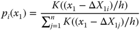
of ![]() with respect to the Lebesgue measure can be estimated using the kernel estimator
with respect to the Lebesgue measure can be estimated using the kernel estimator ![]() . The kernel density estimator is defined in (3.43). The density
. The kernel density estimator is defined in (3.43). The density ![]() of the martingale measure with respect to the Lebesgue measure can be estimated as
of the martingale measure with respect to the Lebesgue measure can be estimated as
Figure 13.1(a) shows the estimate ![]() of the density of the martingale measure with respect to the physical measure (red). The blue curve shows the density of the risk neutral log-normal density with respect to the estimated physical measure. We see that the measures put more probability mass on the negative increments than the physical measure. Fitting of a log-normal distribution is discussed in the connection of Figure 3.11.23 Panel (b) shows the kernel estimate
of the density of the martingale measure with respect to the physical measure (red). The blue curve shows the density of the risk neutral log-normal density with respect to the estimated physical measure. We see that the measures put more probability mass on the negative increments than the physical measure. Fitting of a log-normal distribution is discussed in the connection of Figure 3.11.23 Panel (b) shows the kernel estimate ![]() of the density of the physical measure as a red curve, and the estimate
of the density of the physical measure as a red curve, and the estimate ![]() of the density of the Esscher martingale measure with respect to the Lebesgue measure as a red dashed curve. We apply the standard normal kernel and the normal reference rule to choose the smoothing parameter. The blue curves show the corresponding densities in the log-normal model.
of the density of the Esscher martingale measure with respect to the Lebesgue measure as a red dashed curve. We apply the standard normal kernel and the normal reference rule to choose the smoothing parameter. The blue curves show the corresponding densities in the log-normal model.

Figure 13.1 Esscher martingale measure: One Period. (a) The density of the Esscher martingale measure (red) and the density of the risk neutral log-normal measure (blue). The densities are with respect to the physical measure. (b) The kernel density estimate of the physical measure (red), and the corresponding Esscher martingale measure (red dashed). The log-normal physical measure (blue), and the corresponding risk neutral log-normal density (dashed blue).
Figure 13.2 shows density ratios. Panel (a) shows the ratio

and panel (b) shows the ratios

where ![]() is an estimate of the log-normal physical measure,
is an estimate of the log-normal physical measure, ![]() is an estimate of the log-normal risk neutral measure, and
is an estimate of the log-normal risk neutral measure, and  .
.

Figure 13.2 Esscher martingale measure: Density ratios in one period. (a) The density estimate of the Esscher martingale measure divided by the density estimate of the log-normal martingale measure. (b) The density estimate of the physical measure divided by the estimate log-normal physical measure (solid). The dashed line shows the ratio of the corresponding risk neutral densities.
A Martingale Measure for S&P 500: Two Periods
Let us estimate the Esscher martingale measure for the two period model with two periods of 10 days. Let
be the price increments. Our S&P 500 data provides a sample of identically distributed observations of ![]() . The observations are
. The observations are
where
where ![]() . We use nonoverlapping increments. Let
. We use nonoverlapping increments. Let

where ![]() is the sample average of
is the sample average of ![]() , and
, and ![]() is the minimizer of
is the minimizer of ![]() over
over ![]() . Let
. Let

where ![]() is the minimizer of
is the minimizer of ![]() over
over ![]() , and
, and ![]() is a regression estimate evaluated at
is a regression estimate evaluated at ![]() , when the response variable is
, when the response variable is ![]() and the explanatory variable is
and the explanatory variable is ![]() . We apply a kernel regression estimate of (6.20) and (6.21) to define
. We apply a kernel regression estimate of (6.20) and (6.21) to define

where ![]() ,
, ![]() , are the observation of
, are the observation of ![]() ,
,
are the kernel weights, ![]() is the Gaussian kernel function and
is the Gaussian kernel function and ![]() is the smoothing parameter, chosen by the normal reference rule.
is the smoothing parameter, chosen by the normal reference rule.
The density ![]() of the martingale measure with respect to the underlying physical measure of
of the martingale measure with respect to the underlying physical measure of ![]() can be estimated as
can be estimated as
We can also assume the independence of the increments and estimate ![]() by
by
Figure 13.3 shows estimates of the density of the Esscher measure with respect to the physical measure. In panel (a) we show estimate (13.15), which does not assume independence, and in panel (b) we show estimate (13.16), which assumes independence.
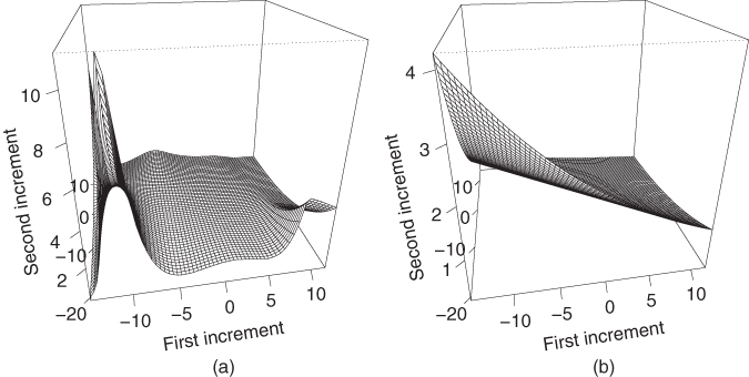
Figure 13.3 Esscher martingale measure: Two Periods. Estimates of the density of the Esscher measure with respect to the physical measure. (a) Increments are assumed to be dependent. (b) Increments are assumed to be independent.
13.2.3.4 Examples of Equivalent Martingale Measures
We calculate the class of equivalent martingale measures in the one period binary model, in the one period ternary model, and in the one period model with a finite amount of states, which generalizes the two previous models.
The One Period Binary Model
Let us have two assets: bond ![]() and stock
and stock ![]() . The value of the bond at time 1 is
. The value of the bond at time 1 is ![]() , where
, where ![]() . The value of the stock at time 1 is
. The value of the stock at time 1 is ![]() with probability
with probability ![]() and
and ![]() with probability
with probability ![]() , where
, where ![]() and
and ![]() . That is,
. That is,
Let the price of the bond be ![]() and the price of the stock be
and the price of the stock be ![]() . Let us consider probability measure
. Let us consider probability measure ![]() which is defined by
which is defined by
where ![]() . If
. If ![]() is a martingale measure, then it satisfies
is a martingale measure, then it satisfies
This holds if
Thus, there exists an equivalent martingale measure if and only if
Thus, the market is arbitrage-free if and only if (13.18) holds. The martingale measure is unique. The calculation will be repeated in (14.18), where derivative pricing is discussed.24 Note that the pricing in the binary model was already studied in (13.1).
The One Period Ternary Model
Let us have two assets: bond ![]() and stock
and stock ![]() . The value of the bond at time 1 is
. The value of the bond at time 1 is ![]() , where
, where ![]() . The value of the stock at time 1 is
. The value of the stock at time 1 is ![]() with probability
with probability ![]() ,
, ![]() with probability
with probability ![]() , and
, and ![]() with probability
with probability ![]() , where
, where ![]() , and
, and ![]() . That is,
. That is,
Let the price of the bond be ![]() and the price of the stock be
and the price of the stock be ![]() . Let us consider probability measure
. Let us consider probability measure ![]() , which is defined by
, which is defined by
where ![]() and
and ![]() . If
. If ![]() is a martingale measure, then it satisfies
is a martingale measure, then it satisfies
This holds if ![]() , where
, where
We can write

Thus, there exists an equivalent martingale measure if and only if
Thus, the market is arbitrage-free if and only if (13.20) holds. There are several martingale measures.25
A Finite Amount of States
Let us consider the one period model with a finite amount of states. Now the probability space ![]() has a finite number of elements. We have
has a finite number of elements. We have ![]() basic securities and
basic securities and ![]() possible states. In the binary model
possible states. In the binary model ![]() . In the ternary model
. In the ternary model ![]() and
and ![]() .
.
The ![]() th risky asset
th risky asset ![]() takes
takes ![]() values, corresponding to the
values, corresponding to the ![]() different states. Let
different states. Let ![]() be the
be the ![]() matrix whose elements are
matrix whose elements are ![]() , where
, where ![]() is the
is the ![]() th state and
th state and ![]() is the
is the ![]() th risky asset.
th risky asset.
Let ![]() be the
be the ![]() vector of the probabilities of the
vector of the probabilities of the ![]() states. Let
states. Let ![]() be the
be the ![]() vector of the prices of the risky assets at time 0. Let
vector of the prices of the risky assets at time 0. Let ![]() be the vector of the risky assets.
be the vector of the risky assets.
Let ![]() be a
be a ![]() vector of probabilities of the
vector of probabilities of the ![]() states. Vector
states. Vector ![]() is a martingale measure if
is a martingale measure if
We can assume that ![]() and
and ![]() , because the redundant basic assets can be removed. A redundant asset would correspond to a column of
, because the redundant basic assets can be removed. A redundant asset would correspond to a column of ![]() which could be expressed as a linear combination of the other columns.
which could be expressed as a linear combination of the other columns.
When ![]() , then there exists a unique equivalent martingale measure, and this is the solution to (13.21):
, then there exists a unique equivalent martingale measure, and this is the solution to (13.21):
When ![]() , then the system (13.21) of
, then the system (13.21) of ![]() linear equations with
linear equations with ![]() variables has many solutions.
variables has many solutions.
13.2.4 European Contingent Claims
13.2.4.1 The Definition of an European Continent Claim
We use the terms “contingent claim” and “derivative” interchangeably. However, these terms can have a different meaning.
- 1. A European contingent claim is a nonnegative random variable
 defined on the probability space
  .
. - 2. A derivative of the underlying assets
 is a European contingent claim, which is measurable with respect to the
  -algebra
  generated by the price process
  ,
,  .
.
We assume that ![]() , and thus in our case the two definitions lead to the same concept. Time
, and thus in our case the two definitions lead to the same concept. Time ![]() is called the maturity, or the expiration date.26 The examples of European contingent claims include the following.
is called the maturity, or the expiration date.26 The examples of European contingent claims include the following.
- 1. A call and a put on the
 th asset are defined by

- where
 is the strike price and
  .
. - 2. An Asian call and put option are defined by

- where

 , and
, and  is the cardinality of
  .
.- 3. A knock-out option on the
 th asset is defined by
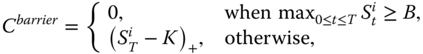
- where
 is the strike price, and
  is the barrier.
13.2.4.2 Arbitrage-Free Prices of European Continent Claims
A European contingent claim ![]() is attainable (replicable, redundant), if there exists a self-financing trading strategy
is attainable (replicable, redundant), if there exists a self-financing trading strategy ![]() whose terminal portfolio value is equal to
whose terminal portfolio value is equal to ![]() :
:
The trading strategy ![]() is called a replicating strategy for
is called a replicating strategy for ![]() . A contingent claim is attainable if and only if the discounted claim
. A contingent claim is attainable if and only if the discounted claim

has the form

for a self-financing trading strategy ![]() with value process
with value process ![]() . Now it is natural to take the initial value
. Now it is natural to take the initial value
to be the fair price of ![]() , because a different price would lead to an arbitrage opportunity. The corresponding arbitrage-free price of the contingent claim
, because a different price would lead to an arbitrage opportunity. The corresponding arbitrage-free price of the contingent claim ![]() is
is
We need to define an arbitrage-free price also for those contingent claims which are not attainable. In fact, in typical market models a contingent claim cannot be replicated. Föllmer and Schied (2002, p. 238) formulate the following definition. An arbitrage-free price of a discounted claim ![]() is a real number
is a real number ![]() , if there exists an adapted stochastic process
, if there exists an adapted stochastic process ![]() such that
such that
- 1.
 ,
, - 2.
 for
for  ,
, - 3.
 , and
, and - 4. the enlarged market model with price process
 is arbitrage-free.
According to this definition, an arbitrage-free price of a contingent claim is such that trading with this price at time 0 does not allow an arbitrage opportunity. A corresponding arbitrage-free price of the continent claim ![]() is then
is then
We can express the class of arbitrage-free prices with the help of equivalent martingale measures. Föllmer and Schied (2002, Theorem 5.30, p. 239) formulate the following theorem.
The price of contingent claim ![]() can now be written as
can now be written as

In the Black–Scholes model we use continuous compounding, where ![]() , and
, and ![]() , so that for a call option
, so that for a call option ![]() ; see (14.47). In many cases we denote by
; see (14.47). In many cases we denote by ![]() the time of writing the option and then
the time of writing the option and then ![]() , so that
, so that ![]() .
.
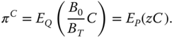
13.2.4.3 Pricing Kernel
The pricing kernel (discount factor) ![]() , related to the martingale measure
, related to the martingale measure ![]() , is defined as the discounted density of
, is defined as the discounted density of ![]() with respect to the physical measure
with respect to the physical measure ![]() :
:

The price of ![]() is given in (13.23) as
is given in (13.23) as ![]() . Now the price of derivative
. Now the price of derivative ![]() can be written as
can be written as
The One Period Binary Model
In the one period binary model, the martingale measure was defined as the measure
where the probability ![]() is defined in (13.17). The pricing kernel is function
is defined in (13.17). The pricing kernel is function ![]() , defined by
, defined by

Let ![]() be a derivative, where
be a derivative, where ![]() . The price of
. The price of ![]() is
is
A Finite Amount of States
Let us continue to study the one period model with a finite amount of states. Let ![]() be the
be the ![]() vector of the probabilities of the
vector of the probabilities of the ![]() states. Let
states. Let ![]() be the
be the ![]() vector of the prices of the risky assets at time 0. Let
vector of the prices of the risky assets at time 0. Let ![]() be the vector of the risky assets. Let
be the vector of the risky assets. Let ![]() be the
be the ![]() matrix whose elements are the values
matrix whose elements are the values ![]() of the
of the ![]() th asset at the
th asset at the ![]() th state.
th state.
Let ![]() be an equivalent martingale measure, which is a solution to the equation in (13.21). In the case
be an equivalent martingale measure, which is a solution to the equation in (13.21). In the case ![]() we may obtain
we may obtain ![]() from (13.22) as
from (13.22) as ![]() . Let
. Let
for ![]() . Let
. Let ![]() be a derivative. The price of
be a derivative. The price of ![]() is
is

The Arrow–Debreu securities take value 1 in one state and value 0 in other states: for the ![]() th Arrow–Debreu security
th Arrow–Debreu security ![]() it holds that
it holds that ![]() , and
, and ![]() for
for ![]() . Then
. Then ![]() is the
is the ![]() identity matrix. Then
identity matrix. Then ![]() and
and ![]() .27
.27
13.2.5 Completeness
The second fundamental theorem of asset pricing says that every European contingent claim can be attained (replicated) if and only if there exists a unique equivalent martingale measure. If every contingent claim can be attained, then every contingent claim has a unique arbitrage-free price and every contingent claim can be hedged perfectly. The case that there is only one equivalent martingale measure occurs never in practice, but it is possible to be close to this situation.
An arbitrage-free market model is called complete if every European contingent claim is attainable. Now we state the second fundamental theorem of asset pricing.
A proof can be found in Föllmer and Schied (2002, Theorem 5.38, p. 245), where an additional statement is proved: In a complete market, the number of atoms in ![]() is bounded above by
is bounded above by ![]() .28
.28
Let us give examples related to completeness.
13.2.5.1 The One Period Binary Model
In the one period binary model, we have two assets: bond ![]() and stock
and stock ![]() . The bond satisfies
. The bond satisfies ![]() , where
, where ![]() . The stock satisfies
. The stock satisfies
where ![]() and
and ![]() . Let the price of the bond be
. Let the price of the bond be ![]() and the price of the stock be
and the price of the stock be ![]() . The space of attainable payoffs is
. The space of attainable payoffs is
Let us consider contingent claim ![]() , where
, where ![]() . To replicate the contingent claim, we need to choose
. To replicate the contingent claim, we need to choose ![]() and
and ![]() so that
so that
This leads to equations

We have two equations and two free variables. The model is complete.
13.2.5.2 The One Period Ternary Model
Let us have two assets: bond ![]() and stock
and stock ![]() . The bond satisfies
. The bond satisfies ![]() , where
, where ![]() . The stock satisfies
. The stock satisfies
where ![]() , and
, and ![]() . Let the price of the bond be
. Let the price of the bond be ![]() and the price of the stock be
and the price of the stock be ![]() . The space of attainable payoffs is
. The space of attainable payoffs is
Let us consider contingent claim ![]() , where
, where ![]() . To replicate the contingent claim, we need to choose
. To replicate the contingent claim, we need to choose ![]() and
and ![]() so that
so that
This leads to equations
We have three equations and two free variables. The model is not complete.
13.2.5.3 A Finite Amount of States
Let us continue to study the one period model with a finite amount of states. Let ![]() be the
be the ![]() vector of the probabilities of the
vector of the probabilities of the ![]() states. Let
states. Let ![]() be the
be the ![]() vector of the prices of the risky assets at time 0. Let
vector of the prices of the risky assets at time 0. Let ![]() be the vector of the risky assets. Let
be the vector of the risky assets. Let ![]() be the
be the ![]() matrix whose elements are the values
matrix whose elements are the values ![]() of the
of the ![]() th asset at the
th asset at the ![]() th state.
th state.
We can assume that ![]() and
and ![]() , because the redundant basic assets can be removed. A redundant asset would correspond to a column of
, because the redundant basic assets can be removed. A redundant asset would correspond to a column of ![]() which could be expressed as a linear combination of the other columns. A redundant basic asset could be considered as a derivative.
which could be expressed as a linear combination of the other columns. A redundant basic asset could be considered as a derivative.
A derivative security is random variable ![]() which takes
which takes ![]() possible values. Let those values be in
possible values. Let those values be in ![]() vector
vector ![]() . To replicate
. To replicate ![]() , we need to find
, we need to find ![]() vector
vector ![]() so that
so that ![]() . This leads to the matrix equation
. This leads to the matrix equation
When ![]() , then
, then
When ![]() , then we do not always have a solution, because there are
, then we do not always have a solution, because there are ![]() free variables and
free variables and ![]() equations.
equations.
We can choose an approximate replication by minimizing the sum of squared replication errors. Let the replication error be
where ![]() is the Euclidean norm in
is the Euclidean norm in ![]() . The minimizer is
. The minimizer is
which is the same formula as the formula for the least squares coefficients in the linear regression ![]() . Note that
. Note that ![]() matrix
matrix ![]() has rank
has rank ![]() , when
, when ![]() has rank
has rank ![]() , and thus
, and thus ![]() is invertible.
is invertible.
The Arrow–Debreu securities provide an example of derivatives. An Arrow–Debreu security has price 1 in one state and 0 in the other states. There are as many Arrow–Debreu securities as there are states. When ![]() , the columns of
, the columns of ![]() give the portfolio weights for replicating the Arrow–Debreu securities.
give the portfolio weights for replicating the Arrow–Debreu securities.
13.2.6 American Contingent Claims
An American contingent claim is defined as a non-negative adapted process
on the filtered space ![]() . The random variable
. The random variable ![]() is the payoff if the American option is exercised at time
is the payoff if the American option is exercised at time ![]() . For example, in the case of the American call option with strike price
. For example, in the case of the American call option with strike price ![]() ,
, ![]() , where
, where ![]() is the price of the underlying asset at time
is the price of the underlying asset at time ![]() .
.
The buyer of an American contingent claim has the right to choose the exercise time ![]() . The buyer receives the amount
. The buyer receives the amount ![]() at time
at time ![]() .
.
A stopping time is a random variable ![]() taking values in
taking values in ![]() such that
such that ![]() for
for ![]() . An exercise strategy is a stopping time taking values in
. An exercise strategy is a stopping time taking values in ![]() . The payoff obtained by using
. The payoff obtained by using ![]() is equal to
is equal to ![]() . We denote with
. We denote with ![]() the set of exercise strategies.
the set of exercise strategies.
13.2.6.1 European and Bermudan Options
An European contingent claim is obtained as a special case of an American contingent claim, when we choose ![]() for
for ![]() . The value of the American option is larger or equal to the value of the corresponding European option.
. The value of the American option is larger or equal to the value of the corresponding European option.
A Bermudan option can be exercised at times ![]() . Formally we can define a Bermudan contingent claim as a non-negative adapted process
. Formally we can define a Bermudan contingent claim as a non-negative adapted process ![]() ,
, ![]() , on the filtered space
, on the filtered space ![]() . A Bermudan option can be obtained as an American option with
. A Bermudan option can be obtained as an American option with ![]() for
for ![]() .
.
On the other hand, an American option can be considered as a special case of a Bermudan option with ![]() . Also, from the point of view of the continuous time model with time space
. Also, from the point of view of the continuous time model with time space ![]() , an American option in a discrete time model could be considered as a Bermudan option whose possible exercise times are
, an American option in a discrete time model could be considered as a Bermudan option whose possible exercise times are ![]() .
.
13.2.6.2 The Set of Arbitrage-Free Prices
Let ![]() be a discounted American claim and let
be a discounted American claim and let ![]() be the payoff which is obtained for a fixed exercise strategy
be the payoff which is obtained for a fixed exercise strategy ![]() . Now
. Now ![]() can be considered as a discounted European contingent claim, whose set of arbitrage-free prices is given in Theorem 13.2 as
can be considered as a discounted European contingent claim, whose set of arbitrage-free prices is given in Theorem 13.2 as
Föllmer and Schied (2002, Definition 6.31) give the following definition for an arbitrage-free price. A number ![]() is called an arbitrage-free price of a discounted American claim
is called an arbitrage-free price of a discounted American claim ![]() if
if
- 1.
There exists some
 and
and  such that
  .
.(The price
 is not too high.)
 - 2.
There does not exist
 such that
  for all
  .
.(The price
 is not too low.)
The set of arbitrage-free prices is characterized in Föllmer and Schied (2002, Theorem 6.33). It is assumed that ![]() for all
for all ![]() and
and ![]() . The set
. The set ![]() of arbitrage-free prices is an interval with endpoints
of arbitrage-free prices is an interval with endpoints ![]() and
and ![]() , where
, where

The interval can be a single point, open, or half open.
13.2.6.3 Exercise Strategies for the Buyer
Let us call an exercise strategy ![]() optimal if
optimal if
where

Thus, an exercise strategy is defined to be optimal, if it maximizes the expectation among the class ![]() of the payoffs. Note that the definition can be generalized so that we maximize
of the payoffs. Note that the definition can be generalized so that we maximize ![]() , where
, where ![]() is a utility function, and
is a utility function, and ![]() is a probability measure, possibly different from the physical measure
is a probability measure, possibly different from the physical measure ![]() .
.
Föllmer and Schied (2002, Theorem 6.20) shows that the exercise strategy ![]() is optimal, when we define
is optimal, when we define
where

It is assumed that ![]() for
for ![]() . Process
. Process ![]() is called a Snell envelope of
is called a Snell envelope of ![]() with respect to the measure
with respect to the measure ![]() . Föllmer and Schied (2002, Proposition 6.22) notes that any optimal exercise strategy
. Föllmer and Schied (2002, Proposition 6.22) notes that any optimal exercise strategy ![]() satisfies
satisfies ![]() , so that
, so that ![]() is the minimal optimal exercise strategy.
is the minimal optimal exercise strategy.
Föllmer and Schied (2002, Theorem 6.23) shows that ![]() is also an optimal exercise strategy, when we define
is also an optimal exercise strategy, when we define
where ![]() means
means ![]() . In addition,
. In addition, ![]() is the largest optimal exercise strategy in the sense that any optimal exercise strategy
is the largest optimal exercise strategy in the sense that any optimal exercise strategy ![]() satisfies
satisfies ![]() .
.
13.2.6.4 American Options in Complete Models
Let us assume that the market model is complete, so that there exists the unique equivalent martingale measure ![]() . We defined the optimal exercise time in (13.24) using the physical measure
. We defined the optimal exercise time in (13.24) using the physical measure ![]() , and the construction of the optimal exercise time was made in (13.25) using the physical measure
, and the construction of the optimal exercise time was made in (13.25) using the physical measure ![]() . Let us define the Snell envelope
. Let us define the Snell envelope ![]() using the equivalent martingale measure
using the equivalent martingale measure ![]() . The value
. The value ![]() can be considered as the unique arbitrage-free price, because
can be considered as the unique arbitrage-free price, because
holds ![]() -almost surely, when
-almost surely, when ![]() is optimal with respect to
is optimal with respect to ![]() ; see Föllmer and Schied (2002, Corollary 6.24).
; see Föllmer and Schied (2002, Corollary 6.24).
13.3 Evaluation of Pricing and Hedging Methods
The evaluation of option pricing and hedging can be done either from the point of view of the writer or from the point of view of the buyer. The writer's point of view is to minimize the hedging error, or to optimize the return of the hedging portfolio. The buyer's point of view is to find fair prices for options. For example, the buyer could be interested whether the buying of the options leads to abnormal returns, as compared to the returns of the underlying.
13.3.1 The Wealth of the Seller
We assume that the seller (writer) of the option hedges the position, and thus the wealth of the seller of the option at the expiration is equal to the hedging error. The writer receives the option premium, makes self-financed trading to replicate the option, and pays the terminal value of the option. We consider the pricing to be fair and the hedging to be effective if the distribution of the hedging error (replication error) is as concentrated around zero as possible. However, we have to study separately the negative hedging errors (losses) and the positive hedging errors (gains).
13.3.1.1 Hedging Error
The hedging error ![]() of the writer of the option is obtained from (13.10) as
of the writer of the option is obtained from (13.10) as
where

Here the risk free rate is ![]() ,
, ![]() is the price of the option,
is the price of the option, ![]() is the terminal value of the option,
is the terminal value of the option, ![]() are the hedging coefficients,
are the hedging coefficients, ![]() are the stock prices, the current time is denoted by 0, the time to expiration is
are the stock prices, the current time is denoted by 0, the time to expiration is ![]() days, and hedging is done daily.
days, and hedging is done daily.
13.3.1.2 Historical Simulation
We denote the time series of observed historical daily prices by ![]() . We construct
. We construct ![]() sequences of prices:
sequences of prices:
where
for ![]() . Each sequence has length
. Each sequence has length ![]() and the initial price in each sequence is
and the initial price in each sequence is ![]() . We estimate the distribution of the hedging error
. We estimate the distribution of the hedging error ![]() from the observations
from the observations
where ![]() is computed from the prices
is computed from the prices ![]() .
.
An example of a computation of hedging errors is given in (14.81), where Black-Scholes hedging is applied with sequential sample standard deviations as the volatility estimates. See also (14.80), where Black-Scholes hedging is applied with non-sequential sample standard deviations as the volatility estimates.
13.3.1.3 Comparison of the Error Distributions
We estimate the distribution of the hedging error ![]() using data
using data ![]() . A graphical summary of the error distribution is obtained by using tail plots and kernel density estimation, for example.
. A graphical summary of the error distribution is obtained by using tail plots and kernel density estimation, for example.
The Mean of Squared Hedging Errors
In quadratic hedging the purpose is to minimize the mean squared hedging errors ![]() ; see Section 15.1 and Chapter 16. Thus it is natural to estimate the quality of a hedging strategy by the sample mean of squared hedging errors
; see Section 15.1 and Chapter 16. Thus it is natural to estimate the quality of a hedging strategy by the sample mean of squared hedging errors

We can decompose the mean into the mean over negative hedging errors and over positive hedging errors:

where
This composition is reasonable because the negative hedging errors are losses for the writer of the option and the positive hedging errors are gains for the writer of the option.
The Expected Utility of the Error Distribution
Even when the purpose of the hedging is typically to minimize the hedging error and not to maximize the wealth of the hedger, it is of interest to study the properties of the wealth distribution from the point of view of portfolio theory. This can be done by estimating the expected utility of the error distribution. We can use the exponential utility function ![]() , where
, where ![]() is the risk aversion parameter. Note that the hedging errors
is the risk aversion parameter. Note that the hedging errors ![]() can take any real value, and thus we cannot apply the power utility functions. The expected utility is estimated by
can take any real value, and thus we cannot apply the power utility functions. The expected utility is estimated by

See Section 9.2.2 for a discussion about expected utility.
13.3.2 The Wealth of the Buyer
We can ignore the hedging of the options and try to evaluate solely the fairness of the price. This approach can be considered to be the approach of the buyer of the option. We have at least the following possibilities.
- 1. Comparison with the market prices. The success of a pricing approach can be evaluated by testing whether the prices of the approach provide a good fit to the observed market prices of the derivatives.
The comparison with the market prices is possible for liquid options. Note that a pricing method for illiquid options can be obtained by calibrating the parameters of the pricing method using liquid options. For example, the implied volatility of Black–Scholes pricing can be obtained from liquid options and then used as the volatility of the Black–Scholes formula to price illiquid options.
- 2. Sharpe ratios. We can estimate the Sharpe ratios of option strategies. The Sharpe ratios obtained by option buying should not be too far away from the Sharpe ratios of the underlying assets. This is illustrated in Section 17.2.3.

and thus the expected gain is
However, a typical price for a Finnish lottery of this type is 0.8 € and playing the game with this entrance price results in the expected loss of 0.67 €. Using the logarithmic utility gives a positive utility

which would give the price of ![]() €. Thus, the market price of a lottery can be justified by pointing out that the market price is equal to the expected utility, for some utility function. Intuitively, a lottery is attractive because it provides an opportunity to a dramatic improvement of wealth, with a negligible price.
€. Thus, the market price of a lottery can be justified by pointing out that the market price is equal to the expected utility, for some utility function. Intuitively, a lottery is attractive because it provides an opportunity to a dramatic improvement of wealth, with a negligible price.

If ![]() is a martingale, then
is a martingale, then ![]() is called a martingale transformation. In our case
is called a martingale transformation. In our case ![]() .
.
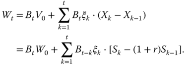

for each ![]() .
.
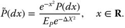

where ![]() is the set of rational numbers and
is the set of rational numbers and ![]() .
.
where ![]() is the convex set of probability measures equivalent to
is the convex set of probability measures equivalent to ![]() and
and ![]() . Now
. Now ![]() . If
. If ![]() , then there is arbitrage. If
, then there is arbitrage. If ![]() , then arbitrage is obtained by borrowing with the risk-free rate and buying the stock. If
, then arbitrage is obtained by borrowing with the risk-free rate and buying the stock. If ![]() , then the arbitrage is obtained by selling the stock short and investing in the risk-free rate.
, then the arbitrage is obtained by selling the stock short and investing in the risk-free rate.
Let ![]() and let
and let ![]() be the vector of
be the vector of ![]() Arrow–Debreu securities Then,
Arrow–Debreu securities Then, ![]() , and
, and ![]() , where
, where ![]() is the
is the ![]() th state,
th state, ![]() .
.