
Chapter 17
Option Strategies
Optionscan be used to create almost any type of a profit function. Trading with stocks allows the possibility of short selling and leveraging, but options open up a huge number of possibilities for creating a payoff that suits the expectations and the risk profile of an investor. For example, a protective put can be used to protect a portfolio of stocks from negative returns, and a straddle can be used to profit simultaneously from large positive and large negative returns of the stock.
We describe option strategies in three ways: the profit function, the return function, and the return distribution. The profit function shows the profit of the option strategy at the expiration, as a function of the value of the underlying. For example, the profit function of a long call strategy is equal to
where ![]() is the stock price at the expiration,
is the stock price at the expiration, ![]() is the strike price,
is the strike price, ![]() is the premium of the call, and
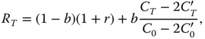
is the premium of the call, and ![]() is the interest rate.1 The return function shows the gross return of the option strategy. For example, the return function of a long call strategy is given by
is the interest rate.1 The return function shows the gross return of the option strategy. For example, the return function of a long call strategy is given by

The return distribution means the probability distribution of the return of the option strategy. For example, the return distribution of a long call strategy is the probability distribution of the random variable ![]() . The probability distribution can be described by the distribution function, which in this case is
. The probability distribution can be described by the distribution function, which in this case is
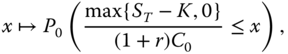
where ![]() , and
, and ![]() is the conditional probability, conditional on the information available at time 0. The probability distribution of the option return depends on the conditional probability distribution of the underlying
is the conditional probability, conditional on the information available at time 0. The probability distribution of the option return depends on the conditional probability distribution of the underlying ![]() , and this probability distribution is unknown. We use both the histogram estimator and the tail plot of the empirical distribution function to estimate the unknown return distribution of the option.
, and this probability distribution is unknown. We use both the histogram estimator and the tail plot of the empirical distribution function to estimate the unknown return distribution of the option.
The method of using the return distribution (17.3) is the most intuitive and useful to describe an option strategy, from the three methods (17.1)–(17.3). In fact, the return distribution of the option is directly relevant for the investor who considers including options into the portfolio. On the other hand, the use of the return distribution involves both the problem of estimating the probability distribution and the problem of visualizing the probability distribution.
Option strategies provide an instructive case study for the performance measurement. We get more insight into such concepts as Sharpe ratio, cumulative wealth, and risk aversion by studying the performance measurement of option strategies, instead of just studying the performance measurement of portfolios of stocks.
Section 17.1 shows profit functions of option strategies, which include vertical spreads, strangles, straddles, butterflies, condors, calendar spreads, covered calls, and protective puts. Section 17.2 shows return functions and return distributions of the option strategies, and measures the performance of the option strategies.
17.1 Option Strategies
It is possible to create a large number of profit functions by combining calls and puts with different strike prices and expiration dates. Our examples include vertical spreads, strangles, straddles, butterflies, condors, and calendar spreads. In addition, we discuss how to combine options with the underlying to create protective puts and covered calls.
17.1.1 Calls, Puts, and Vertical Spreads
Calls and puts are the basic building blocks for creating profit functions. Vertical spreads are combinations of calls and puts that limit the downside risk of selling pure calls and puts.
17.1.1.1 Calls and Puts
Figure 17.1(a)–(d) shows profit functions of a long call, long put, short call, and short put. For a call, the profit function is
where ![]() is the stock price at the expiration,
is the stock price at the expiration, ![]() is the strike price,
is the strike price, ![]() is the premium of the call, and
is the premium of the call, and ![]() is the interest rate. For the put, the profit function is
is the interest rate. For the put, the profit function is
where ![]() is the premium of the put. When a call is bought, the maximum profit is unlimited. When a put is bought, the maximum profit is equal to the strike price minus the premium. The losses are limited both when a call is bought and when a put is bought.2
is the premium of the put. When a call is bought, the maximum profit is unlimited. When a put is bought, the maximum profit is equal to the strike price minus the premium. The losses are limited both when a call is bought and when a put is bought.2

Figure 17.1 Profit functions. (a) Long call; (b) long put; (c) short call; (d) short put; (e) short call spread; (f) short put spread; (g) long call spread; (h) long put spread; (i) long  ratio call spread; (j) long
  ratio put spread; (k) long call ladder; and (l) long put ladder.
17.1.1.2 Vertical Spreads
Figure 17.1(e)–(h) shows profit functions of a short call spread, short put spread, long call spread. and long put spread. Let the strike prices satisfy ![]() . Vertical spreads are the following trades:
. Vertical spreads are the following trades:
- 1. Short call spread. Short
 call, long
  call.
call. - 2. Short put spread. Long
 put, short
  put.
put. - 3. Long call spread. Long
 call, short
  call.
call. - 4. Long put spread. Short
 put, long
  put.
put.
A short call spread has a special importance, because this trade allows us to sell a call option but it makes the maximum possible loss limited, because a call with a higher strike price is bought simultaneously. Selling a put has a limited loss but a short put spread makes the maximum possible loss smaller; see (17.13).
Figure 17.1(i)–(l) shows profit functions of a long ![]() ratio call spread, long
ratio call spread, long ![]() ratio put spread, long call ladder, and long put ladder. Ratio spreads are generalizations of simple vertical spreads. Ladders are examples of combinations of three options. The strike prices satisfy
ratio put spread, long call ladder, and long put ladder. Ratio spreads are generalizations of simple vertical spreads. Ladders are examples of combinations of three options. The strike prices satisfy ![]() . Ratio spreads and ladders are defined as follows:
. Ratio spreads and ladders are defined as follows:
- 1. Long
 ratio call spread. Short
  call, long 2 times
  call. (Also called a call backspread.)
 - 2. Long
 ratio put spread. Long 2 times
  put, short
  put. (Also called a put backspread.)
 - 3. Long call ladder. Long
 call, short
  call, short
  call.
call. - 4. Long put ladder. Short
 put, short
  put, long
  put.
put.
17.1.2 Strangles, Straddles, Butterflies, and Condors
Figure 17.2(a)–(d) shows profit functions of a long straddle, long strangle, long butterfly, and long condor.

Figure 17.2 Profit functions. (a) Long straddle; (b) long strangle; (c) long butterfly; and (d) long condor.
Long straddles and strangles are profitable when the underlying makes a large move.
- 1. Long straddle. Long
 put and long
  call, where
  is close to the current stock price.
 - 2. Long strangle. The profit function of a long strangle can be constructed in two ways. Let
 and let
  be the current stock price.
- a. Long strangle. Long
 put, long
  call.
call. - b. Long guts. Long
 call, long
  put.
put.
- a. Long strangle. Long
Straddles are special cases of strangles and guts: when ![]() , then we obtain a straddle from a strangle or from a guts.
, then we obtain a straddle from a strangle or from a guts.
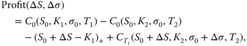
Figure 17.3 shows a two-dimensional profit function of a straddle. Now we consider the profit not as a univariate function of the price of the underlying, but as a two-dimensional function of the change in the price of the underlying and of the change in the volatility. The Black–Scholes prices are used to define the profit function. Panel (a) shows a perspective plot of function

where ![]() and
and ![]() are the Black–Scholes prices at time
are the Black–Scholes prices at time ![]() of a call and a put, when the underlying has value
of a call and a put, when the underlying has value ![]() , strike price is
, strike price is ![]() ,
, ![]() is the annualized volatility, and
is the annualized volatility, and ![]() is the time of expiration. Panel (b) shows slices
is the time of expiration. Panel (b) shows slices
for five values of ![]() . We can see that a long straddle profits also from a rising volatility, and not only from large moves of the underlying.
. We can see that a long straddle profits also from a rising volatility, and not only from large moves of the underlying.

Figure 17.3 A profit function of a straddle. (a) A perspective plot of function  , defined in (17.4); (b) slices
  for five values of
  .
.
To profit when the underlying does not move, one can sell a straddle, strangle, or guts. However, these trades have an unlimited downside. Thus, it is useful to apply butterflies and condors, which have a limited downside. Below ![]() .
.
- 1. Long butterflies can be constructed in three ways:
- a. Call butterfly. Long
 call, short two
  calls, long
  call.
call. - b. Put butterfly. Long
 put, short two
  puts, long
  put.
put. - c. Long iron butterfly. Long
 put, short
  put and call, long
  call.3
- a. Call butterfly. Long
- 2. Long condors can be constructed in three ways:
- a. Call condor. Long
 call, short
  call, short
  call, long
  call.
call. - b. Put condor. Long
 put, short
  put, short
  put, long
  put.
put. - c. Long iron condor. Long
 put, short
  call, short
  put, long
  call.
call.
- a. Call condor. Long
A long butterfly is obtained from a long condor by taking ![]() . Selling a strangle can be considered as obtainable from a condor by letting
. Selling a strangle can be considered as obtainable from a condor by letting ![]() and
and ![]() . Selling a straddle can be considered as obtainable from a butterfly by letting
. Selling a straddle can be considered as obtainable from a butterfly by letting ![]() and
and ![]() .
.
17.1.3 Calendar Spreads
Calendar spreads allow us to profit from a rising volatility by shorting an option with a shorter time to expiration and going long for an option with a longer time to expiration. Calendar spreads are also called “time spreads” and “horizontal spreads.” Diagonal calendar spreads make a simultaneous bet for the direction of the underlying.
- 1. Long calendar spread:
- a. Call calendar spread. Short
 call, long
  call.
call. - b. Put calendar spread. Short
 put, long
  put.
put. - c. Long straddle calendar spread. Short
 straddle, long
  straddle.
- a. Call calendar spread. Short
- 2. Long diagonal calendar spread:
- a. Call diagonal calendar spread. Short
 ,
,  call, long
  ,
,  call.
call. - b. Put diagonal calendar spread. Short
 ,
,  put, long
  ,
,  put.
put. - c. Long diagonal straddle calendar spread. Short
 ,
,  straddle, long
  ,
,  straddle.
- a. Call diagonal calendar spread. Short
Figure 17.4 shows a profit function of call calendar spread. The profit function is a function of two variables: the change in stock price and the change in volatility. At time 0 we short a call with maturity ![]() and buy a call with maturity
and buy a call with maturity ![]() . The trade is terminated at
. The trade is terminated at ![]() . Panel (a) shows a perspective plot and panel (b) shows slices
. Panel (a) shows a perspective plot and panel (b) shows slices ![]() for five values of
for five values of ![]() . The profit function is
. The profit function is

where ![]() is the Black–Scholes price at time
is the Black–Scholes price at time ![]() of a call option when
of a call option when ![]() is the stock price,
is the stock price, ![]() is the strike price,
is the strike price, ![]() is the annualized volatility, and
is the annualized volatility, and ![]() is the expiration time. Here
is the expiration time. Here ![]() , so that we have
, so that we have ![]() .
.
Figure 17.5 shows a profit function of call diagonal calendar spread. At time 0 we short a call with maturity ![]() and strike
and strike ![]() , and buy a call with maturity
, and buy a call with maturity ![]() and strike
and strike ![]() . The trade is terminated at
. The trade is terminated at ![]() . Panel (a) shows a perspective plot and panel (b) shows slices
. Panel (a) shows a perspective plot and panel (b) shows slices ![]() for five values of
for five values of ![]() . The profit function is
. The profit function is
where ![]() .
.

Figure 17.4 Profit of calendar. (a) A perspective plot; (b) slices.
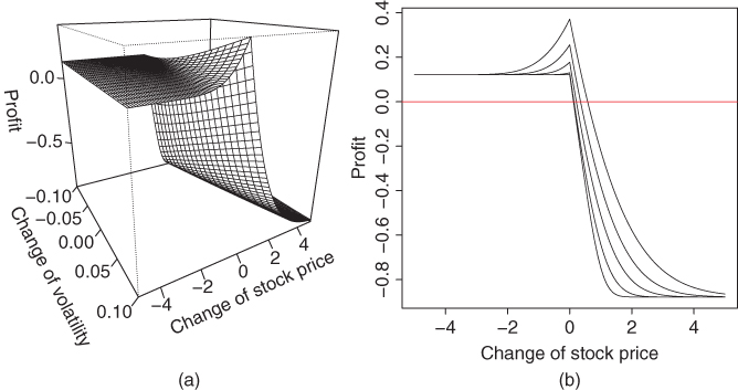
Figure 17.5 Profit of diagonal calendar. (a) A perspective plot; (b) slices.
17.1.4 Combining Options with Stocks and Bonds
A stock can be replicated by a combination of a call and a put. Furthermore, options can be combined with the underlying to make a protective put and a covered call. A bond and a call can be combined to create a position with bounded losses but a stock type upside potential.
17.1.4.1 Replication of the Underlying
The payout of buying a ![]() -call and simultaneously selling a
-call and simultaneously selling a ![]() -put is
-put is ![]() :
:
The profit of buying a ![]() -call and simultaneously selling a
-call and simultaneously selling a ![]() -put is
-put is
where ![]() and
and ![]() are the premiums of the call and the put.
are the premiums of the call and the put.
Choosing ![]() leads to the profit
leads to the profit
Indeed, a forward contract to buy stock at time ![]() for the price
for the price ![]() is equivalent to buying a
is equivalent to buying a ![]() -call and simultaneously selling
-call and simultaneously selling ![]() -put. This is the so called put–call parity
-put. This is the so called put–call parity
studied in Section 14.1.2. Thus, when ![]() , the profit of buying a
, the profit of buying a ![]() -call and simultaneously selling a
-call and simultaneously selling a ![]() -put is
-put is ![]() , because the put–call parity gives
, because the put–call parity gives ![]() . Thus, the payoff of a stock can be obtained by options.
. Thus, the payoff of a stock can be obtained by options.
Conversely, being long ![]() -put and short
-put and short ![]() -call, where
-call, where ![]() , is a bet on a falling stock price.4
, is a bet on a falling stock price.4
Figure 17.6(a) and (b) shows profit functions of replicating being long and being short of a stock.

Figure 17.6 Profit functions. (a) Long stock; (b) short stock; (c) protective put; (d) covered call; (e) covered shorting; and (f) bond and call.
17.1.4.2 Protective Put and Covered Call
A protective put consists of a simultaneous buying of the underlying and a put on the underlying. The strike price of the put is ![]() , where
, where ![]() is the current price of the underlying. This position gives insurance against a falling price of the underlying, with the cost of paying the premium for the put option.
is the current price of the underlying. This position gives insurance against a falling price of the underlying, with the cost of paying the premium for the put option.
A covered call consists of a simultaneous buying of the underlying and selling a call with strike price ![]() . A covered call has less risk than the pure position in the underlying, because a premium is obtained from selling the call. On the other hand, selling the call limits the potential upside. Note that a covered call has a similarity with a long call spread.
. A covered call has less risk than the pure position in the underlying, because a premium is obtained from selling the call. On the other hand, selling the call limits the potential upside. Note that a covered call has a similarity with a long call spread.
A covered shorting consists of a simultaneous selling of the underlying and buying a call with strike price ![]() . A covered shorting has less risk than plain shorting, because buying the call makes the loss bounded from below.
. A covered shorting has less risk than plain shorting, because buying the call makes the loss bounded from below.
Figure 17.6 shows profit functions of a protective put, covered call, and covered shorting in panels (c)–(e).
17.1.4.3 A Bond and A Call
Let a bond and a call be such that the maturity date of the bond is the same as the expiration date of the call. Buying a bond and a call leads to a position where the guaranteed return is smaller than from the pure bond position, because the premium for buying the call has to be subtracted from the profit. On the other hand, there is a considerable upside potential, unlike in the case of the pure bond position. The combination leads to a capital guarantee product.
Figure 17.6(f) shows a profit function of buying a bond and a call. We assume that the profit from the bond is higher than the premium of the call, and thus the profit is always positive. Thus the profit function of Figure 17.6(f) differs from the profit function of the call in Figure 17.1(a), where a loss is possible.
17.2 Profitability of Option Strategies
We discuss how to study the profitability of option strategies that were defined in Section 17.1. First we list the returns of option strategies, then we study the distributions of the returns of the option strategies, and finally compute Sharpe ratios of the option strategies.
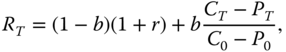
What is the gross return of an option strategy? An option strategy is defined by giving its payoff

where ![]() , and
, and ![]() are the payoffs of options. For example, the payoff of a long call spread is
are the payoffs of options. For example, the payoff of a long call spread is
where ![]() ,
, ![]() , and
, and ![]() . Let us include the possibility of investing in the risk-free rate, and let
. Let us include the possibility of investing in the risk-free rate, and let ![]() be the risk-free rate for the period
be the risk-free rate for the period ![]() . Let
. Let ![]() be the premiums of the options. When
be the premiums of the options. When ![]() , then we can assume without losing generality that
, then we can assume without losing generality that

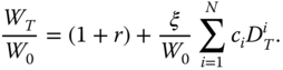
Then the return of the strategy in (17.5) can be written as

where ![]() is the weight of the risk-free rate and
is the weight of the risk-free rate and ![]() is the weight of the option strategy.
is the weight of the option strategy.
The return can be also written as

where

A third way to write the return is

where
In (17.6), (17.7), (17.8), we have assumed that ![]() . In the case when
. In the case when ![]() , we can combine the option strategy with the risk-free return. We start with the initial wealth
, we can combine the option strategy with the risk-free return. We start with the initial wealth ![]() and obtain the wealth
and obtain the wealth

where ![]() is the exposure to the option strategy. The return is
is the exposure to the option strategy. The return is
Note that (17.8) leads to (17.9) with ![]() .
.
17.2.1 Return Functions of Option Strategies
We draw return functions
where ![]() is the gross return of the option strategy. We denote the strike prices
is the gross return of the option strategy. We denote the strike prices
We use the following notation for the payoffs of calls:
We use the following notation for the payoffs of puts:
The corresponding premiums are ![]() ,
, ![]() ,
, ![]() and
and ![]() ,
, ![]() ,
, ![]()
We draw a blue horizontal line at the level one, because the gross return one means that the wealth does not change. We draw a red horizontal line at the height zero, because in the case of stock trading the gross return zero means bankruptcy. Note that in option trading we interpret the negative gross return as leading to debt, and the amount deposited in the margin account should be used to pay this debt.
The premiums are chosen to be the Black–Scholes prices, with the annualized volatility ![]() . The interest rate is
. The interest rate is ![]() . The initial stock price is
. The initial stock price is ![]() . The time to expiration is 6 months (which is
. The time to expiration is 6 months (which is ![]() in fractions of a year).
in fractions of a year).
17.2.1.1 Calls, Puts, and Vertical Spreads
Figure 17.7(a) shows return functions of buying and selling calls. The gross return is

where ![]() and
and ![]() . We show functions for the weights
. We show functions for the weights ![]() ,
, ![]() ,
, ![]() , and
, and ![]() . The profit functions of buying and selling calls are shown in Figure 17.1(a) and (c).
. The profit functions of buying and selling calls are shown in Figure 17.1(a) and (c).
Figure 17.7(b) shows return functions of buying and selling puts. The gross return is

where ![]() and
and ![]() . We show functions for the weights
. We show functions for the weights ![]() ,
, ![]() ,
, ![]() , and
, and ![]() . The profit functions of buying and selling puts are shown in Figure 17.1(b) and (d).
. The profit functions of buying and selling puts are shown in Figure 17.1(b) and (d).
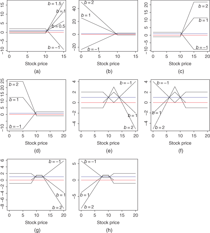
Figure 17.7 Return functions of calls, puts, and vertical spreads. (a) Long and short call; (b) long and short put; (c) long and short call spread; (d) long and short put spread; (e) short  ratio call spread; (f) short
  ratio put spread; (g) long call ladder; and (h) long put ladder.
Figure 17.7(c) shows return functions of call vertical spreads. The gross return is

where ![]() ,
, ![]() , and
, and ![]() . When
. When ![]() , we obtain a long call spread. When
, we obtain a long call spread. When ![]() we obtain a short call spread. The corresponding profit functions are shown in Figure 17.1(e) and (g). It is of interest to note that a short call vertical spread has a return function which is bounded from below. Indeed, we have that
we obtain a short call spread. The corresponding profit functions are shown in Figure 17.1(e) and (g). It is of interest to note that a short call vertical spread has a return function which is bounded from below. Indeed, we have that ![]() .5
Thus, when
.5
Thus, when ![]() ,
,

Figure 17.7(d) shows return functions of put vertical spreads. The gross return is

where ![]() ,
, ![]() , and
, and ![]() . When
. When ![]() , we obtain a long put spread. When
, we obtain a long put spread. When ![]() we obtain a short put spread. The corresponding profit functions are shown in Figure 17.1(f) and (h). It is of interest to calculate the lower bound for the return of a short put vertical spread. We have that
we obtain a short put spread. The corresponding profit functions are shown in Figure 17.1(f) and (h). It is of interest to calculate the lower bound for the return of a short put vertical spread. We have that ![]() . Thus, when
. Thus, when ![]() ,
,

Figure 17.7(e) shows return functions of ![]() ratio call spreads. The gross return is
ratio call spreads. The gross return is
where ![]() ,
, ![]() , and
, and ![]() . When
. When ![]() , we obtain a short
, we obtain a short ![]() ratio call spread. When
ratio call spread. When ![]() we obtain a long
we obtain a long ![]() ratio call spread. The profit function of a long
ratio call spread. The profit function of a long ![]() ratio call spread is shown in Figure 17.1(i).
ratio call spread is shown in Figure 17.1(i).
Figure 17.7(f) shows return functions of ![]() ratio put spreads. The gross return is
ratio put spreads. The gross return is

where ![]() ,
, ![]() , and
, and ![]() . When
. When ![]() , we obtain a short
, we obtain a short ![]() ratio put spread. When
ratio put spread. When ![]() we obtain a long
we obtain a long ![]() ratio put spread. The profit function of a long
ratio put spread. The profit function of a long ![]() ratio put spread is shown in Figure 17.1(j).
ratio put spread is shown in Figure 17.1(j).
Figure 17.7(g) shows return functions of call ladders. The gross return is

where ![]() ,
, ![]() ,
, ![]() , and
, and ![]() . When
. When ![]() , we obtain a long call ladder. When
, we obtain a long call ladder. When ![]() we obtain a short call ladder. The profit function of a long call ladder is shown in Figure 17.1(k).
we obtain a short call ladder. The profit function of a long call ladder is shown in Figure 17.1(k).
Figure 17.7(h) shows return functions of put ladders. The gross return is

where ![]() ,
, ![]() ,
, ![]() , and
, and ![]() . When
. When ![]() , we obtain a long put ladder. When
, we obtain a long put ladder. When ![]() we obtain a short put ladder. The profit function of a long put ladder is shown in Figure 17.1(l).
we obtain a short put ladder. The profit function of a long put ladder is shown in Figure 17.1(l).
17.2.1.2 Straddles, Strangles, Butterflys, and Condors
Figure 17.8(a) and (b) shows return functions of straddles and strangles. The gross return is

where ![]() and
and ![]() . In panel (a) we have straddles:
. In panel (a) we have straddles: ![]() . In panel (b) we have strangles:
. In panel (b) we have strangles: ![]() . When
. When ![]() , we obtain a long straddle and strangle. When
, we obtain a long straddle and strangle. When ![]() we obtain a short straddle and strangle. The profit functions of a long straddle and a long strangle are shown in Figure 17.2(a) and (b).
we obtain a short straddle and strangle. The profit functions of a long straddle and a long strangle are shown in Figure 17.2(a) and (b).

Figure 17.8 Return functions of straddles, strangles, butterflies, and condors. (a) Long and short straddles; (b) long and short strangles; (c) long and short butterflies; and (d) long and short condors.
Figure 17.8(c) and (d) shows return functions of call butterflies and condors. The gross return is

where ![]() ,
, ![]() ,
, ![]() , and
, and ![]() . In panel (b) we have butterflies:
. In panel (b) we have butterflies: ![]() . In panel (c) we have condors:
. In panel (c) we have condors: ![]() . When
. When ![]() , we obtain a long butterfly and a long condor. When
, we obtain a long butterfly and a long condor. When ![]() we obtain a short butterfly and a short condor. The profit functions of a long butterfly and a long condor are shown in Figure 17.2(c) and (d).
we obtain a short butterfly and a short condor. The profit functions of a long butterfly and a long condor are shown in Figure 17.2(c) and (d).
17.2.1.3 Combining Options with Stocks and Bonds
Options can be combined with the underlying to replicate the underlying, to apply a protective put, and to construct a covered call and a covered short. Furthermore, options can be combined with bonds.
Replication of a Stock
Let us replicate the stock by a simultaneous buying of a ![]() -call and
-call and ![]() -put. The put–call parity implies that the prices
-put. The put–call parity implies that the prices ![]() and
and ![]() of the options satisfy
of the options satisfy
see (14.8) for a discussion of the put–call parity. When ![]() , then
, then ![]() , and the return is
, and the return is
where ![]() .
.
When ![]() , then we can define the return using (17.9) as
, then we can define the return using (17.9) as
where ![]() .
.
Figure 17.9(a) shows the return function ![]() for the return (17.18), when
for the return (17.18), when ![]() . Note that Figure 17.6(a) and (b) shows profit functions of being long and being short of a stock.
. Note that Figure 17.6(a) and (b) shows profit functions of being long and being short of a stock.

Figure 17.9 Return functions of combination trades. (a) Replication of stock; (b) protective put; (c) covered shorting; and (d) bond and call.
A Protective Put
A protective put is a position where the buying of the underlying is combined with buying a put with a strike price ![]() . Let us consider more generally the return
. Let us consider more generally the return

A protective put is obtained when ![]() .
.
Figure 17.9(b) shows a return function of a protective put. In fact, we show the cases ![]() ,
, ![]() , and
, and ![]() .
.
We can calculate a lower bound to the return of a protective put. In fact,6
When ![]() , the return satisfies
, the return satisfies

A Covered Call and a Covered Short
A covered call is a position where the buying of the underlying is combined with selling a call with a strike price ![]() . A covered short is a position where the shorting of a stock is combined by the buying of a call with strike price
. A covered short is a position where the shorting of a stock is combined by the buying of a call with strike price ![]() .
.
Let us consider returns

A covered call is obtained when ![]() . A covered short is obtained when
. A covered short is obtained when ![]() . Figure 17.9(c) shows return functions for the cases
. Figure 17.9(c) shows return functions for the cases ![]() ,
, ![]() , and
, and ![]() .
.
Selling a stock has an unbounded maximum loss but in a covered short we buy simultaneously a call option, with strike price ![]() , which makes the maximum possible loss bounded. Selling a call has an unbounded maximum loss but in a covered call we buy simultaneously the stock, which makes the loss bounded when the stock price goes up, although it is possible to lose the total investment, when the stock price goes to zero. The strike price of the covered call satisfies
, which makes the maximum possible loss bounded. Selling a call has an unbounded maximum loss but in a covered call we buy simultaneously the stock, which makes the loss bounded when the stock price goes up, although it is possible to lose the total investment, when the stock price goes to zero. The strike price of the covered call satisfies ![]() . The covered call can be used to earn extra return when the stock price does not make a big upside move. We have that7
. The covered call can be used to earn extra return when the stock price does not make a big upside move. We have that7
When ![]() , the return satisfies
, the return satisfies

and thus the return of the covered short is bounded from below. When ![]() , the return satisfies
, the return satisfies

and thus the return of the covered call is bounded from above.
A Bond and a Call
A suitable simultaneous buying of a bond and a call creates a capital guarantee product. We assume that the time to maturity of the bond and the time to the expiration of the call are equal. The return is given in (17.10) by

where ![]() ,
, ![]() is the premium of the call, and
is the premium of the call, and ![]() is the net return of the bond. Unlike in (17.10) we take
is the net return of the bond. Unlike in (17.10) we take ![]() close to zero, in order to guarantee that the capital is not lost.
close to zero, in order to guarantee that the capital is not lost.
Figure 17.9(d) shows return functions for the cases ![]() ,
, ![]() , and
, and ![]() .
.
17.2.2 Return Distributions of Option Strategies
We estimate the return distributions using the S&P 500 daily data, described in Section 2.4.1. The daily data is aggregated to have sampling interval of 20 trading days, and we study options with the time to expiration being 20 days.
The option prices are taken to be the Black–Scholes prices with the volatility being the annualized sample standard deviation of the complete time series of the observations. The risk-free rate is taken to be zero. These simplifications do not prevent us from gaining qualitative insight into the return distributions. The Black–Scholes prices are different from the real market prices, and thus we are not able to obtain precise estimates of the actual return distributions of the past option returns. In particular, the out-of-the-money options tend to have higher market prices than the Black–Scholes prices: this can be seen from the volatility smile, which means that the implied volatilities of the out-of-the-money options have larger implied volatilities than the at-the-money options (see Section 14.3.2).
To estimate the return distributions we use histogram and kernel estimators, as defined in Section 3.2.2. We use the normal reference rule to choose the smoothing parameter of the kernel density estimator. Also, we apply tail plots of the empirical distribution function, as defined in Section 3.2.1.
17.2.2.1 Calls, Puts, and Vertical Spreads
Figure 17.10 shows a return distribution of buying a call option with moneyness ![]() . The return is given in (17.10), where we choose
. The return is given in (17.10), where we choose ![]() . Panel (a) shows a histogram estimate of the call returns. The red curve shows a kernel estimate of the corresponding S&P 500 returns. Panel (b) shows a tail plot of the empirical distribution function of the option returns with black circles. The red circles show a tail plot of the empirical distribution function of the corresponding S&P 500 returns. The corresponding profit function is shown in Figure 17.1(a) and the return function is shown in Figure 17.7(a). We see that there is a large probability of gross return zero, and small probabilities of high returns.
. Panel (a) shows a histogram estimate of the call returns. The red curve shows a kernel estimate of the corresponding S&P 500 returns. Panel (b) shows a tail plot of the empirical distribution function of the option returns with black circles. The red circles show a tail plot of the empirical distribution function of the corresponding S&P 500 returns. The corresponding profit function is shown in Figure 17.1(a) and the return function is shown in Figure 17.7(a). We see that there is a large probability of gross return zero, and small probabilities of high returns.

Figure 17.10 Long call option: Return distribution. (a) A histogram estimate of call returns (black) and a kernel estimate of S&P 500 returns (red); (b) an empirical distribution function of option returns (black) and S&P 500 returns (red).
Figure 17.11 shows the return distribution of buying a put option with moneyness ![]() . The return is given in (17.11), where we choose
. The return is given in (17.11), where we choose ![]() . Panel (a) shows a histogram estimate of the put returns. The red curve shows a kernel estimate of the corresponding S&P 500 returns. Panel (b) shows a tail plot of the option returns (black) and a tail plot of the corresponding S&P 500 returns (red). The corresponding profit function is shown in Figure 17.1(b) and the return function is shown in Figure 17.7(b). We see that the return distribution of buying a put option is close to the return distribution of buying a call option.
. Panel (a) shows a histogram estimate of the put returns. The red curve shows a kernel estimate of the corresponding S&P 500 returns. Panel (b) shows a tail plot of the option returns (black) and a tail plot of the corresponding S&P 500 returns (red). The corresponding profit function is shown in Figure 17.1(b) and the return function is shown in Figure 17.7(b). We see that the return distribution of buying a put option is close to the return distribution of buying a call option.

Figure 17.11 Long put option: Return distribution. (a) A histogram estimate of call returns (black) and a kernel estimate of S&P 500 returns (red); (b) an empirical distribution function of option returns (black) and S&P 500 returns (red).
Figure 17.12 shows the return distribution of selling a call with moneyness ![]() . The return is given in (17.10), where we choose
. The return is given in (17.10), where we choose ![]() . Panel (a) shows a histogram estimate of the returns. The red curve shows a kernel estimate of the corresponding S&P 500 returns. Panel (b) shows a tail plot of the option returns (black) and a tail plot of the corresponding S&P 500 returns (red). The corresponding profit function is shown in Figure 17.1(c) and the return function is shown in Figure 17.7(a). We see that the return distribution of selling a call option is a mirror image of the return distribution of buying a call option: there is a large probability of a gross return over one, but small probabilities of quite large negative returns.
. Panel (a) shows a histogram estimate of the returns. The red curve shows a kernel estimate of the corresponding S&P 500 returns. Panel (b) shows a tail plot of the option returns (black) and a tail plot of the corresponding S&P 500 returns (red). The corresponding profit function is shown in Figure 17.1(c) and the return function is shown in Figure 17.7(a). We see that the return distribution of selling a call option is a mirror image of the return distribution of buying a call option: there is a large probability of a gross return over one, but small probabilities of quite large negative returns.

Figure 17.12 Short call option: Return distribution. (a) A histogram estimate of option returns (black) and a kernel estimate of S&P 500 returns (red); (b) an empirical distribution function of option returns (black) and S&P 500 returns (red).
Figure 17.13 shows the return distribution of selling a put option with moneyness ![]() . The return is given in (17.11), where we choose
. The return is given in (17.11), where we choose ![]() . Panel (a) shows a histogram estimate of the returns. The red curve shows a kernel estimate of the corresponding S&P 500 returns. Panel (b) shows a tail plot of the option returns (black) and a tail plot of the corresponding S&P 500 returns (red). The corresponding profit function is shown in Figure 17.1(d) and the return function is shown in Figure 17.7(b). We see that the return distribution of selling a put option is close to the return distribution of selling a call option.
. Panel (a) shows a histogram estimate of the returns. The red curve shows a kernel estimate of the corresponding S&P 500 returns. Panel (b) shows a tail plot of the option returns (black) and a tail plot of the corresponding S&P 500 returns (red). The corresponding profit function is shown in Figure 17.1(d) and the return function is shown in Figure 17.7(b). We see that the return distribution of selling a put option is close to the return distribution of selling a call option.

Figure 17.13 Short put option: Return distribution. (a) A histogram estimate of option returns (black) and a kernel estimate of S&P 500 returns (red); (b) an empirical distribution function of option returns (black) and S&P 500 returns (red).
Figure 17.14 shows the return distribution of selling a call spread with ![]() ,
, ![]() , and
, and ![]() . The return is given in (17.12), where we take
. The return is given in (17.12), where we take ![]() . Panel (a) shows a histogram estimate of the returns. The red curve shows a kernel estimate of the corresponding S&P 500 returns. Panel (b) shows a tail plot of the option returns (black) and a tail plot of the corresponding S&P 500 returns (red). The corresponding profit function is shown in Figure 17.1(e) and the return function is shown in Figure 17.7(c). The return distribution is bounded from below, unlike in the case of Figure 17.12, where a call option is sold.
. Panel (a) shows a histogram estimate of the returns. The red curve shows a kernel estimate of the corresponding S&P 500 returns. Panel (b) shows a tail plot of the option returns (black) and a tail plot of the corresponding S&P 500 returns (red). The corresponding profit function is shown in Figure 17.1(e) and the return function is shown in Figure 17.7(c). The return distribution is bounded from below, unlike in the case of Figure 17.12, where a call option is sold.

Figure 17.14 Selling a call spread: Return distribution. (a) A histogram estimate of option returns (black) and a kernel estimate of S&P 500 returns (red); (b) an empirical distribution function of option returns (black) and S&P 500 returns (red).
Figure 17.15 shows the return distribution of a ![]() ratio call spread with
ratio call spread with ![]() ,
, ![]() , and
, and ![]() . The return is given in (17.14), where we take
. The return is given in (17.14), where we take ![]() . Panel (a) shows a histogram estimate of the return distribution of the option. The red curve shows a kernel estimate of the corresponding S&P 500 returns. Panel (b) shows a tail plot of the option returns (black) and a tail plot of the corresponding S&P 500 returns (red). The corresponding profit function of long position is shown in Figure 17.1(i) and the return function is shown in Figure 17.7(e).
. Panel (a) shows a histogram estimate of the return distribution of the option. The red curve shows a kernel estimate of the corresponding S&P 500 returns. Panel (b) shows a tail plot of the option returns (black) and a tail plot of the corresponding S&P 500 returns (red). The corresponding profit function of long position is shown in Figure 17.1(i) and the return function is shown in Figure 17.7(e).

Figure 17.15 A  ratio call spread: Return distribution. (a) A histogram estimate of option returns (black) and a kernel estimate of S&P 500 returns (red); (b) an empirical distribution function of option returns (black) and S&P 500 returns (red).
Figure 17.16 shows the return distribution of a short call ladder with ![]() ,
, ![]() ,
, ![]() , and
, and ![]() . The return is given in (17.15), where we take
. The return is given in (17.15), where we take ![]() . Panel (a) shows a histogram estimate of the return distribution of the option. The red curve shows a kernel estimate of the corresponding S&P 500 returns. Panel (b) shows a tail plot of the option returns (black) and a tail plot of the corresponding S&P 500 returns (red). The corresponding profit function of a long position is shown in Figure 17.1(k) and the return function is shown in Figure 17.7(g).
. Panel (a) shows a histogram estimate of the return distribution of the option. The red curve shows a kernel estimate of the corresponding S&P 500 returns. Panel (b) shows a tail plot of the option returns (black) and a tail plot of the corresponding S&P 500 returns (red). The corresponding profit function of a long position is shown in Figure 17.1(k) and the return function is shown in Figure 17.7(g).

Figure 17.16 A short call ladder: Return distribution. (a) A histogram estimate of option returns (black) and a kernel estimate of S&P 500 returns (red); (b) an empirical distribution function of option returns (black) and S&P 500 returns (red).
17.2.2.2 Straddles, Strangles, Butterflys, and Condors
Figure 17.17 shows the return distribution of a straddle with ![]() and
and ![]() . The return is given in (17.16), where we take
. The return is given in (17.16), where we take ![]() . Panel (a) shows a histogram estimate of the return distribution of the option strategy. The red curve shows a kernel estimate of the corresponding S&P 500 returns. Panel (b) shows a tail plot of the option strategy returns (black) and a tail plot of the corresponding S&P 500 returns (red). The corresponding profit function of a long position is shown in Figure 17.2(a) and the return function is shown in Figure 17.8(a).
. Panel (a) shows a histogram estimate of the return distribution of the option strategy. The red curve shows a kernel estimate of the corresponding S&P 500 returns. Panel (b) shows a tail plot of the option strategy returns (black) and a tail plot of the corresponding S&P 500 returns (red). The corresponding profit function of a long position is shown in Figure 17.2(a) and the return function is shown in Figure 17.8(a).

Figure 17.17 A straddle: Return distribution. (a) A histogram estimate of option returns (black) and a kernel estimate of S&P 500 returns (red); (b) an empirical distribution function of option returns (black) and S&P 500 returns (red).
Figure 17.18 shows a short straddle. The setting is the same as in Figure 17.17.

Figure 17.18 A short straddle: Return distribution. (a) A histogram estimate of option returns (black) and a kernel estimate of S&P 500 returns (red); (b) an empirical distribution function of option returns (black) and S&P 500 returns (red).
Figure 17.19 shows the return distribution of a strangle with ![]() ,
, ![]() , and
, and ![]() . The return is given in (17.16), where we take
. The return is given in (17.16), where we take ![]() . Panel (a) shows a histogram estimate of the return distribution of the option strategy. The red curve shows a kernel estimate of the corresponding S&P 500 returns. Panel (b) shows a tail plot of the option strategy returns (black) and a tail plot of the corresponding S&P 500 returns (red). The corresponding profit function of a long position is shown in Figure 17.2(b) and the return function is shown in Figure 17.8(b).
. Panel (a) shows a histogram estimate of the return distribution of the option strategy. The red curve shows a kernel estimate of the corresponding S&P 500 returns. Panel (b) shows a tail plot of the option strategy returns (black) and a tail plot of the corresponding S&P 500 returns (red). The corresponding profit function of a long position is shown in Figure 17.2(b) and the return function is shown in Figure 17.8(b).
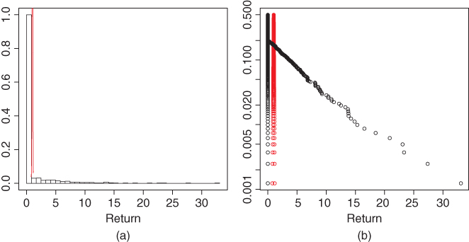
Figure 17.19 A strangle: Return distribution. (a) A histogram estimate of option returns (black) and a kernel estimate of S&P 500 returns (red); (b) an empirical distribution function of option returns (black) and S&P 500 returns (red).
Figure 17.20 shows a short strangle. The setting is the same as in Figure 17.19.

Figure 17.20 A short strangle: Return distribution. (a) A histogram estimate of option returns (black) and a kernel estimate of S&P 500 returns (red); (b) an empirical distribution function of option returns (black) and S&P 500 returns (red).
Figure 17.21 shows the return distribution of a butterfly with ![]() ,
, ![]() ,
, ![]() , and
, and ![]() . The return is given in (17.17), where we take
. The return is given in (17.17), where we take ![]() . Panel (a) shows a histogram estimate of the return distribution of the option strategy. The red curve shows a kernel estimate of the corresponding S&P 500 returns. Panel (b) shows a tail plot of the option strategy returns (black) and a tail plot of the corresponding S&P 500 returns (red). The corresponding profit function of a long position is shown in Figure 17.2(c) and the return function is shown in Figure 17.8(c).
. Panel (a) shows a histogram estimate of the return distribution of the option strategy. The red curve shows a kernel estimate of the corresponding S&P 500 returns. Panel (b) shows a tail plot of the option strategy returns (black) and a tail plot of the corresponding S&P 500 returns (red). The corresponding profit function of a long position is shown in Figure 17.2(c) and the return function is shown in Figure 17.8(c).

Figure 17.21 A butterfly: Return distribution. (a) A histogram estimate of option returns (black) and a kernel estimate of S&P 500 returns (red); (b) an empirical distribution function of option returns (black) and S&P 500 returns (red).
Figure 17.22 shows the return distribution of a short butterfly. The setting is the same as in Figure 17.21.

Figure 17.22 A short butterfly: Return distribution. (a) A histogram estimate of option returns (black) and a kernel estimate of S&P 500 returns (red); (b) an empirical distribution function of option returns (black) and S&P 500 returns (red).
Figure 17.23 shows the return distribution of a condor with ![]() ,
, ![]() ,
, ![]() ,
, ![]() , and
, and ![]() . The return is given in (17.17), where we take
. The return is given in (17.17), where we take ![]() . Panel (a) shows a histogram estimate of the return distribution of the option strategy. The red curve shows a kernel estimate of the corresponding S&P 500 returns. Panel (b) shows a tail plot of the option strategy returns (black) and a tail plot of the corresponding S&P 500 returns (red). The corresponding profit function of a long position is shown in Figure 17.2(d) and the return function is shown in Figure 17.8(d).
. Panel (a) shows a histogram estimate of the return distribution of the option strategy. The red curve shows a kernel estimate of the corresponding S&P 500 returns. Panel (b) shows a tail plot of the option strategy returns (black) and a tail plot of the corresponding S&P 500 returns (red). The corresponding profit function of a long position is shown in Figure 17.2(d) and the return function is shown in Figure 17.8(d).

Figure 17.23 A condor: Return distribution. (a) A histogram estimate of option returns (black) and a kernel estimate of S&P 500 returns (red); (b) an empirical distribution function of option returns (black) and S&P 500 returns (red).
Figure 17.24 shows the return distribution of a short condor. The setting is the same as in Figure 17.23.

Figure 17.24 A short condor: Return distribution. (a) A histogram estimate of option returns (black) and a kernel estimate of S&P 500 returns (red); (b) an empirical distribution function of option returns (black) and S&P 500 returns (red).
17.2.2.3 A Protective Put and a Covered Call
Figure 17.25 shows the return distribution of a protective put with ![]() and
and ![]() . The return is given in (17.20), where we take
. The return is given in (17.20), where we take ![]() . Panel (a) shows a histogram estimate of the return distribution of the option strategy. The red curve shows a kernel estimate of the corresponding S&P 500 returns. Panel (b) shows a tail plot of the option strategy returns (black) and a tail plot of the corresponding S&P 500 returns (red). The corresponding profit function is shown in Figure 17.6(c) and the return function is shown in Figure 17.9(c).
. Panel (a) shows a histogram estimate of the return distribution of the option strategy. The red curve shows a kernel estimate of the corresponding S&P 500 returns. Panel (b) shows a tail plot of the option strategy returns (black) and a tail plot of the corresponding S&P 500 returns (red). The corresponding profit function is shown in Figure 17.6(c) and the return function is shown in Figure 17.9(c).

Figure 17.25 A protective put: Return distribution. (a) A histogram estimate of option returns (black) and a kernel estimate of S&P 500 returns (red); (b) an empirical distribution function of option returns (black) and S&P 500 returns (red).
Figure 17.26 shows the return distribution of a covered call with ![]() and
and ![]() . The return is given in (17.21), where we take
. The return is given in (17.21), where we take ![]() . Panel (a) shows a histogram estimate of the return distribution of the option strategy. The red curve shows a kernel estimate of the corresponding S&P 500 returns. Panel (b) shows a tail plot of the option strategy returns (black) and a tail plot of the corresponding S&P 500 returns (red). The corresponding profit function is shown in Figure 17.6(d) and the return function is shown in Figure 17.9(d).
. Panel (a) shows a histogram estimate of the return distribution of the option strategy. The red curve shows a kernel estimate of the corresponding S&P 500 returns. Panel (b) shows a tail plot of the option strategy returns (black) and a tail plot of the corresponding S&P 500 returns (red). The corresponding profit function is shown in Figure 17.6(d) and the return function is shown in Figure 17.9(d).

Figure 17.26 A covered call: Return distribution. (a) A histogram estimate of option returns (black) and a kernel estimate of S&P 500 returns (red); (b) an empirical distribution function of option returns (black) and S&P 500 returns (red).
17.2.2.4 A Bond and a Call
Figure 17.27 shows the return distribution of a capital guarantee product with ![]() and
and ![]() . The bond gross return is 1.01. The return is given in (17.22), where we take
. The bond gross return is 1.01. The return is given in (17.22), where we take ![]() . Panel (a) shows a histogram estimate of the return distribution of the option strategy. The red curve shows a kernel estimate of the corresponding S&P 500 returns. Panel (b) shows a tail plot of the option strategy returns (black) and a tail plot of the corresponding S&P 500 returns (red). The corresponding profit function of is shown in Figure 17.6(f) and the return function is shown in Figure 17.9(d).
. Panel (a) shows a histogram estimate of the return distribution of the option strategy. The red curve shows a kernel estimate of the corresponding S&P 500 returns. Panel (b) shows a tail plot of the option strategy returns (black) and a tail plot of the corresponding S&P 500 returns (red). The corresponding profit function of is shown in Figure 17.6(f) and the return function is shown in Figure 17.9(d).

Figure 17.27 A bond and a call: Return distribution. (a) A histogram estimate of strategy returns (black) and a kernel estimate of S&P 500 returns (red); (b) an empirical distribution function of strategy returns (black) and S&P 500 returns (red).
17.2.3 Performance Measurement of Option Strategies
We estimate the Sharpe ratios of few option strategies and show the cumulative wealths and wealth ratios.
We use the S&P 500 daily data, described in Section 2.4.1. The option prices are computed using the Black–Scholes formula, with the volatility equal to the sequentially estimated annualized GARCH(![]() ) volatility. The risk-free rate is deduced from the rate of the one-month Treasury bill, using data described in Section 2.4.3.
) volatility. The risk-free rate is deduced from the rate of the one-month Treasury bill, using data described in Section 2.4.3.
The Sharpe ratios are not equal to the Sharpe ratios which are obtained using the market prices of options. Also, we do not take the transaction costs into account. However, studying the performance of option strategies gives insights into the concepts of performance measurement. Also, we can interpret the results as giving information about the properties of the Black–Scholes prices, since the fair option prices should be such that statistical arbitrage is excluded.
17.2.3.1 Covered Call and Protective Put
Figure 17.28 shows the Sharpe ratios of buying (a) covered call and (b) protective put. The ![]() -axis shows the put moneyness, defined as
-axis shows the put moneyness, defined as ![]() , where
, where ![]() is the strike price and
is the strike price and ![]() is the stock price at the time of the writing of the call option. The
is the stock price at the time of the writing of the call option. The ![]() -axis shows the Sharpe ratio. The time to expiration is 20 days (black), 40 days (red), and 60 days (green). The blue horizontal lines show the Sharpe ratio of S&P 500. We see that the Sharpe ratio of the covered call converges to the Sharpe ratio of the underlying, when the strike price increases, and the Sharpe ratio of the protective put converges to the Sharpe ratio of the underlying, when the strike price decreases.
-axis shows the Sharpe ratio. The time to expiration is 20 days (black), 40 days (red), and 60 days (green). The blue horizontal lines show the Sharpe ratio of S&P 500. We see that the Sharpe ratio of the covered call converges to the Sharpe ratio of the underlying, when the strike price increases, and the Sharpe ratio of the protective put converges to the Sharpe ratio of the underlying, when the strike price decreases.

Figure 17.28 Covered call and protective put: Sharpe ratios. (a) Covered call and (b) protective put. The Sharpe ratios as a function of the put moneyness  , when the time to expiration is 20 (black), 40 (red), and 60 (green) trading days.
Figure 17.29 shows the wealth ratios of buying (a) covered call and (b) protective put. The time to expiration is 20 trading days. The strike price is ![]() for the covered call and
for the covered call and ![]() for the protective put, when the stock price is
for the protective put, when the stock price is ![]() .
.

Figure 17.29 Covered call and protective put: Wealth ratios. (a) Covered call and (b) protective put. We show the time series of wealth of the option divided by the wealth of S&P 500.
17.2.3.2 Calls, Puts, and Capital Guarantee Products
Figure 17.30 shows the Sharpe ratios of buying (a) call options and (b) put options. The ![]() -axis shows the put moneyness, defined as
-axis shows the put moneyness, defined as ![]() , where
, where ![]() is the strike price and
is the strike price and ![]() is the stock price at the time of the writing of the option. The
is the stock price at the time of the writing of the option. The ![]() -axis shows the Sharpe ratio. The time to expiration is 20 days (black), 40 days (red), and 60 days (green). The blue horizontal lines show the Sharpe ratio of S&P 500. We see that the Sharpe ratios of the call options converge to the Sharpe ratio of the underlying, when the strike price approaches zero. The Sharpe ratios of the call options are larger than the Sharpe ratio of the underlying when the moneyness is around zero. The Sharpe ratios of the put options are lower than the Sharpe ratio of the underlying.
-axis shows the Sharpe ratio. The time to expiration is 20 days (black), 40 days (red), and 60 days (green). The blue horizontal lines show the Sharpe ratio of S&P 500. We see that the Sharpe ratios of the call options converge to the Sharpe ratio of the underlying, when the strike price approaches zero. The Sharpe ratios of the call options are larger than the Sharpe ratio of the underlying when the moneyness is around zero. The Sharpe ratios of the put options are lower than the Sharpe ratio of the underlying.

Figure 17.30 Buying calls and puts: Sharpe ratios. (a) Long call and (b) long put. The Sharpe ratios as a function of the moneyness, when the time to expiration is 20 (black), 40 (red), and 60 (green) trading days.

Figure 17.31 Buying a call and a bond: Wealth. (a) Time series of cumulative wealths for  (black),
  (red), and
  (green). The blue curve is the cumulative wealth of S&P 500. (b) Wealth ratios.
Figure 17.31 considers the capital guarantee product, which is constructed by combining a call and a bond to give return

where ![]() is the weight. This return was discussed in (17.22). The Sharpe ratio is given in Figure 17.30(a), because the weight
is the weight. This return was discussed in (17.22). The Sharpe ratio is given in Figure 17.30(a), because the weight ![]() does not change the Sharpe ratio (see Section 10.1.1). We choose
does not change the Sharpe ratio (see Section 10.1.1). We choose ![]() positive but close to zero, in order to guarantee the preservation of the capital. The strike price is
positive but close to zero, in order to guarantee the preservation of the capital. The strike price is ![]() for the call, when the stock price is
for the call, when the stock price is ![]() . The time to expiration is 20 trading days. Panel (a) shows the cumulative wealth for
. The time to expiration is 20 trading days. Panel (a) shows the cumulative wealth for ![]() (black),
(black), ![]() (red), and
(red), and ![]() (green). The blue curve is the cumulative wealth of S&P 500. Panel (b) shows the wealth ratios where the cumulative wealths of the capital guarantee products are divided by the cumulative wealth of S&P 500. We see that when
(green). The blue curve is the cumulative wealth of S&P 500. Panel (b) shows the wealth ratios where the cumulative wealths of the capital guarantee products are divided by the cumulative wealth of S&P 500. We see that when ![]() (green), then the bankruptcy follows quite soon. When
(green), then the bankruptcy follows quite soon. When ![]() (red), then the cumulative wealth is larger than for S&P 500, but with the expense of higher volatility.
(red), then the cumulative wealth is larger than for S&P 500, but with the expense of higher volatility.


