
Chapter 10
Performance Measurement
When the performance of a fund is measured, there is a temptation to look only at the past return on the investment. However, it is important to measure the performance by taking the risk into account. An investor can increase both the expected return and the risk by leveraging, so that it is of interest to find the inherent quality of the fund, and leave the choice of the leveraging factor to the investor. The Sharpe ratio is defined as the ratio of the expected excess return to the standard deviation of the excess return. This is an example of a performance measure that penalizes the expected return with the risk.
The measures of performance are usually single numbers, but we cannot hope to completely reduce the characteristics of a fund into a single number. For example, the Sharpe ratio is a single number, but we obtain more information by giving separately the expected excess return and the standard deviation of the excess return, instead of giving only their ratio.
Section 9.2 discussed the ranking of return distributions from the point of view of portfolio selection. This discussion is relevant for the performance measurement. For example, in portfolio selection we could be interested in the conditional expected utility
where ![]() is a utility function,
is a utility function, ![]() is a return, and the expectation is taken conditionally on the state variable
is a return, and the expectation is taken conditionally on the state variable ![]() having value
having value ![]() . If we would have information about the conditional expected utility of all portfolios, then we could choose an optimal portfolio. When
. If we would have information about the conditional expected utility of all portfolios, then we could choose an optimal portfolio. When ![]() is the return of a fund, then the conditional expected utility characterizes the properties of the fund. However, since the conditional expected utility is a function of
is the return of a fund, then the conditional expected utility characterizes the properties of the fund. However, since the conditional expected utility is a function of ![]() , this is a very complicated way to describe the properties of a fund. We can summarize the performance using a single number, and the unconditional expected utility
, this is a very complicated way to describe the properties of a fund. We can summarize the performance using a single number, and the unconditional expected utility
is a single number summarizing the performance. The unconditional expected utility averages over all states ![]() .
.
Has the past performance of a fund been due to a luck or to a skill? This question could be answered by testing the null hypothesis, which states that the long-time performance of a fund is equal to the performance of a market index. Testing is related to the construction of confidence bands to a performance measure. Hypothesis testing and confidence bands can be used to try to answer the question whether the better performance of a fund, as compared to the performance of another fund, is due to a luck or skill. We address the issue of hypothesis testing and confidence bands only when the Sharpe ratio is the performance measure. We note that the confidence bands tend to be quite wide.
Performance measures are computed using a time period ![]() of historical returns. One has to address the issue whether the choice of the time period of historical returns affects the performance measures. This question is considered in Section 10.5, where we provide tools to simultaneously look at the all possible time intervals contained in
of historical returns. One has to address the issue whether the choice of the time period of historical returns affects the performance measures. This question is considered in Section 10.5, where we provide tools to simultaneously look at the all possible time intervals contained in ![]() . These tools are an alternative to looking at the conditional expectation in (10.1). A problem with the conditional expectations in (10.1) is that we have to choose the conditioning state variables
. These tools are an alternative to looking at the conditional expectation in (10.1). A problem with the conditional expectations in (10.1) is that we have to choose the conditioning state variables ![]() , which is a difficult task, as there is a huge number of potentially useful conditioning variables. When we look at the performance of a fund over all subintervals of
, which is a difficult task, as there is a huge number of potentially useful conditioning variables. When we look at the performance of a fund over all subintervals of ![]() , then we get clues about which conditioning variables are relevant for the performance of the fund. For example, we could find answers to the questions: Does this fund perform well only in the bull markets? Does this fund perform well only when the inflation is high?
, then we get clues about which conditioning variables are relevant for the performance of the fund. For example, we could find answers to the questions: Does this fund perform well only in the bull markets? Does this fund perform well only when the inflation is high?
Section 10.1 considers Sharpe ratio. Section 10.2 considers certainty equivalent. Section 10.3 discusses drawdown. Section 10.4 discusses alpha. Section 10.5 presents graphical tools to help the performance measurement.
10.1 The Sharpe Ratio
First, we give the definition of the Sharpe ratio. Then, we derive confidence intervals for the Sharpe ratio and test the equality of two Sharpe ratios. Finally, we give examples of some other measures of risk-adjusted return.
10.1.1 Definition of the Sharpe Ratio
The Sharpe ratio of a financial asset is defined as the expected excess return divided by the standard deviation of the excess return:1

where ![]() is the return of the asset, and
is the return of the asset, and ![]() is the return of a risk-free investment.
is the return of a risk-free investment.
Note that we have not defined the Sharpe ratio as ![]() , where the conditional expectation and the conditional standard deviation are used. Under this definition, we could write the Sharpe ratio as
, where the conditional expectation and the conditional standard deviation are used. Under this definition, we could write the Sharpe ratio as ![]() , since the risk-free rate for the period
, since the risk-free rate for the period ![]() is not a random variable at time
is not a random variable at time ![]() , and thus it can be dropped from the conditional standard deviation. Instead, we have defined the Sharpe ratio in (10.2) using the unconditional expectation and the unconditional standard deviation, so that the risk-free rate is a random variable.
, and thus it can be dropped from the conditional standard deviation. Instead, we have defined the Sharpe ratio in (10.2) using the unconditional expectation and the unconditional standard deviation, so that the risk-free rate is a random variable.
The return period can be, for example, 1 day, 1 month, or 1 year. The annualized Sharpe ratio is defined as

where ![]() is the return horizon:
is the return horizon: ![]() for daily returns,
for daily returns, ![]() for monthly returns, and so on.2 The Sharpe ratio was defined by Sharpe (1966).
for monthly returns, and so on.2 The Sharpe ratio was defined by Sharpe (1966).
An estimator of the Sharpe ratio is obtained from historical returns ![]() and from historical risk-free rates
and from historical risk-free rates ![]() by replacing the population mean and the population standard deviation by the sample mean and the sample standard deviation:
by replacing the population mean and the population standard deviation by the sample mean and the sample standard deviation:
where

where ![]() is the excess return.
is the excess return.
We can increase as much as we like the expected return of a given asset by leveraging. However, leveraging increases also the risk. The Sharpe ratio is invariant with respect to leveraging. Consider an asset with the expected excess return ![]() and the variance of the excess return
and the variance of the excess return ![]() :
:
where ![]() is the time
is the time ![]() return of the risky asset and
return of the risky asset and ![]() is the risk-free rate. Consider a portfolio of the risky asset and the risk-free rate, where the weight of the original asset is
is the risk-free rate. Consider a portfolio of the risky asset and the risk-free rate, where the weight of the original asset is ![]() and the weight of the risk-free asset is
and the weight of the risk-free asset is ![]() , where
, where ![]() . The return of the portfolio is
. The return of the portfolio is
The excess return of the portfolio is
Thus, ![]() and
and ![]() . Thus,
. Thus,

10.1.2 Confidence Intervals for the Sharpe Ratio
Assume we observe historical excess returns ![]() for
for ![]() . The estimator (10.3) of the Sharpe ratio, when multiplied by the annualizing factor, can be written as
. The estimator (10.3) of the Sharpe ratio, when multiplied by the annualizing factor, can be written as
where


and ![]() . Let us assume that
. Let us assume that
as ![]() , where
, where ![]() and
and ![]() is a
is a ![]() covariance matrix. The central limit theorem (10.5) holds at least when the observed excess returns are independent and identically distributed, and the fourth moment of the excess returns is finite. Independence does not hold for financial returns, but the central limit theorem holds when the returns are weakly dependent, as discussed in Section 3.5.1. An application of the delta-method gives3
covariance matrix. The central limit theorem (10.5) holds at least when the observed excess returns are independent and identically distributed, and the fourth moment of the excess returns is finite. Independence does not hold for financial returns, but the central limit theorem holds when the returns are weakly dependent, as discussed in Section 3.5.1. An application of the delta-method gives3
as ![]() , where
, where ![]() is the gradient, and
is the gradient, and ![]() is the Sharpe ratio. We have that
is the Sharpe ratio. We have that

The boundaries of the confidence interval for the Sharpe ratio ![]() with the confidence level
with the confidence level ![]() are
are
where ![]() is the
is the ![]() -quantile of the standard normal distribution,
-quantile of the standard normal distribution,
and ![]() is an estimator of
is an estimator of ![]() . Indeed,
. Indeed, ![]() where
where ![]() .
.
10.1.2.1 Independent Returns
The central limit theorem (10.5) holds when the observed excess returns are independent and identically distributed, and the fourth moment of the excess returns is finite. In this case the asymptotic covariance matrix is

and estimator ![]() is obtained by using the sample variances and the sample covariance. We can write
is obtained by using the sample variances and the sample covariance. We can write

where ![]() and
and ![]() is defined in (10.4).
is defined in (10.4).
10.1.2.2 Dependent Returns
A central limit theorem holds when the dependence is weak. Let ![]() be a vector time series, where
be a vector time series, where ![]() . A central limit theorem states that
. A central limit theorem states that

where

and the autocovariance matrix ![]() is defined as
is defined as
Note that we used the property ![]() . Weak dependence can be defined in terms of mixing coefficients.4
. Weak dependence can be defined in terms of mixing coefficients.4
To estimate ![]() in (10.8) we use
in (10.8) we use

where

for ![]() , and the weights are defined as
, and the weights are defined as
where ![]() is a kernel function satisfying
is a kernel function satisfying ![]() and
and ![]() for all
for all ![]() . We get the estimator (10.7) by choosing
. We get the estimator (10.7) by choosing ![]() and
and ![]() . We get the estimator
. We get the estimator

by choosing ![]() and
and ![]() . A further example is
. A further example is ![]() and
and ![]() . The idea of using weights in asymptotic covariance estimation can be found in Newey and West (1987).
. The idea of using weights in asymptotic covariance estimation can be found in Newey and West (1987).
10.1.2.3 Confidence Intervals for the S&P 500 Sharpe Ratio
Figure 10.1(a) shows the confidence intervals for the Sharpe ratio of S&P 500 index, when the coverage probability is in the range ![]() . The S&P 500 monthly data is described in Section 2.4.3. We have used the estimator (10.7) of the asymptotic covariance matrix. The
. The S&P 500 monthly data is described in Section 2.4.3. We have used the estimator (10.7) of the asymptotic covariance matrix. The ![]() -axis shows the range of possible values of the Sharpe ratio and the
-axis shows the range of possible values of the Sharpe ratio and the ![]() -axis shows the coverage probabilities of the confidence intervals. The yellow vector shows the point estimate of the Sharpe ratio and the red vectors show the confidence interval with 0.95 coverage.
-axis shows the coverage probabilities of the confidence intervals. The yellow vector shows the point estimate of the Sharpe ratio and the red vectors show the confidence interval with 0.95 coverage.
Figure 10.1(b) studies how the confidence intervals change when we use the autocorrelation robust estimator (10.9) of the asymptotic covariance matrix. We show the ratios ![]() as a function of smoothing parameter, where
as a function of smoothing parameter, where ![]() is defined by (10.6) and by the estimator (10.7) for the covariance matrix, whereas
is defined by (10.6) and by the estimator (10.7) for the covariance matrix, whereas ![]() is defined by (10.6) and by the estimator (10.9) for the covariance matrix. These ratios are equal to the ratios of the lengths of the corresponding confidence intervals. We use the kernel function
is defined by (10.6) and by the estimator (10.9) for the covariance matrix. These ratios are equal to the ratios of the lengths of the corresponding confidence intervals. We use the kernel function ![]() and try values
and try values ![]() . For
. For ![]() the ratio is equal to one, because the estimators for the covariance matrix are equal. We see that taking the autocorrelation into account makes the confidence bands eventually shorter, but for moderate
the ratio is equal to one, because the estimators for the covariance matrix are equal. We see that taking the autocorrelation into account makes the confidence bands eventually shorter, but for moderate ![]() the confidence intervals can be longer, too.
the confidence intervals can be longer, too.

Figure 10.1 Confidence intervals for the S&P 500 Sharpe ratio. (a) Confidence intervals corresponding to a coverage probability in  . The
. The  -axis shows the range of possible values of the Sharpe ratio and the
  -axis shows the coverage probabilities of the confidence intervals. The yellow vertical vector indicates the point estimate of the Sharpe ratio and the red vertical vectors show the confidence interval with
  coverage. (b) The ratios
  as a function of smoothing parameter, where
  is the estimator assuming zero autocorrelation, whereas
  assumes autocorrelation.
10.1.3 Testing the Sharpe Ratio
Let us have two portfolios ![]() and
and ![]() with excess returns
with excess returns ![]() and
and ![]() . We want to test the equality of the Sharpe ratios, so that the null hypothesis is
. We want to test the equality of the Sharpe ratios, so that the null hypothesis is
where ![]() and
and ![]() . Portfolio
. Portfolio ![]() could typically be an actively managed portfolio and portfolio
could typically be an actively managed portfolio and portfolio ![]() could be the benchmark index.
could be the benchmark index.
Let us have historical returns ![]() of portfolio
of portfolio ![]() and historical returns
and historical returns ![]() of portfolio
of portfolio ![]() . We use the test statistics
. We use the test statistics
where ![]() is the estimate of the Sharpe ratio of portfolio
is the estimate of the Sharpe ratio of portfolio ![]() , and
, and ![]() is the estimate of the Sharpe ratio of portfolio
is the estimate of the Sharpe ratio of portfolio ![]() . The test statistics can be written as
. The test statistics can be written as
where

and

Let us assume that
as ![]() , where
, where ![]() and
and ![]() is a
is a ![]() covariance matrix. An application of the delta-method gives
covariance matrix. An application of the delta-method gives
as ![]() , where
, where ![]() is the gradient, and
is the gradient, and ![]() is the difference of the Sharpe ratios. We have that
is the difference of the Sharpe ratios. We have that

When the alternative hypothesis is
then the null hypothesis is rejected for large values of the test statistics ![]() , and thus the
, and thus the ![]() -value for the one-sided test is
-value for the one-sided test is
where ![]() is the distribution function of the standard normal distribution and
is the distribution function of the standard normal distribution and
The estimator ![]() of
of ![]() can be defined similarly as in (10.7) or (10.9). Indeed, under the null hypothesis
can be defined similarly as in (10.7) or (10.9). Indeed, under the null hypothesis ![]() , where
, where ![]() . When the alternative hypothesis is
. When the alternative hypothesis is
then the null hypothesis is rejected for large values of the absolute values of test statistics ![]() , and thus the
, and thus the ![]() -value for the two-sided test is
-value for the two-sided test is ![]() . Indeed, under the null hypothesis
. Indeed, under the null hypothesis ![]() . These tests were defined in Ledoit and Wolf (2008).
. These tests were defined in Ledoit and Wolf (2008).
10.1.3.1 A Test Under Normality
A test for the equality of Sharpe ratios is presented in Jobson and Korkie (1981), with the corrected formula in Memmel (2003). They use the test statistics
where ![]() is the sample mean calculated from
is the sample mean calculated from ![]() ,
, ![]() is the corresponding sample standard deviation,
is the corresponding sample standard deviation, ![]() and
and ![]() are the sample mean and standard deviation calculated from
are the sample mean and standard deviation calculated from ![]() , and
, and

where ![]() is the sample covariance. Under the assumption that the returns are normally distributed, the distribution of the test statistics under the null hypothesis can be approximated by the standard normal distribution:
is the sample covariance. Under the assumption that the returns are normally distributed, the distribution of the test statistics under the null hypothesis can be approximated by the standard normal distribution: ![]() . For the one sided alternative, the null hypothesis is rejected for the large values of the test statistics
. For the one sided alternative, the null hypothesis is rejected for the large values of the test statistics ![]() and thus the
and thus the ![]() -value for the one-sided test is
-value for the one-sided test is ![]() , where
, where ![]() is the distribution function of the standard normal distribution.
is the distribution function of the standard normal distribution.
10.1.4 Other Measures of Risk-Adjusted Return
There exist several performance measures that resemble the Sharpe ratio. These performance measures are defined by dividing a measure for the expected return by a measure for the risk.
10.1.4.1 Information Ratio
The information ratio is defined as

where ![]() is the return of the portfolio and
is the return of the portfolio and ![]() is the return of a benchmark portfolio. Thus, the information ratio is like the Sharpe ratio, but the risk-free rate in the Sharpe ratio is replaced by the return of a benchmark.
is the return of a benchmark portfolio. Thus, the information ratio is like the Sharpe ratio, but the risk-free rate in the Sharpe ratio is replaced by the return of a benchmark.
The benchmark return is the return of an asset that is chosen as the benchmark for the asset manager. S&P 500 could be chosen as a benchmark for a US equity fund and MSCI World could be chosen as a benchmark for a global equity fund investing in developed markets. (MSCI is an acronym for Morgan Stanley Capital International.)
10.1.4.2 Sortino ratio
The Sortino ratio is otherwise similar to Sharpe ratio but the standard deviation is replaced by a lower partial moment, and the risk-free rate is replaced by a constant ![]() . The Sortino ratio is defined as
. The Sortino ratio is defined as

where the lower partial moment of order 2 is defined in (3.15) as
Another version of the Sortino ratio is defined as
where ![]() is a risk-free rate.
is a risk-free rate.
10.1.4.3 Omega Ratio
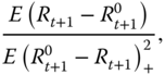
The Omega ratio is the ratio of the upper partial moment of order one to the lower partial moment of order one:

where ![]() is the chosen threshold (the target rate). We have defined the upper and lower partial moments in (3.14) and (3.15). The definition was made in Shadwick and Keating (2002). Note that the Omega ratio is written often using the expressions
is the chosen threshold (the target rate). We have defined the upper and lower partial moments in (3.14) and (3.15). The definition was made in Shadwick and Keating (2002). Note that the Omega ratio is written often using the expressions

and
where ![]() is the distribution function of
is the distribution function of ![]() . The sample Omega ratio is
. The sample Omega ratio is

Another version of the Omega ratio is defined as

where ![]() is a risk-free rate. Note that
is a risk-free rate. Note that ![]() and
and ![]() are close to each other, because probability
are close to each other, because probability ![]() is small.
is small.
10.2 Certainty Equivalent
The certainty equivalent of a return distribution is defined as
where ![]() is a gross return and
is a gross return and ![]() is a utility function. The certainty equivalent is the minimal risk-free rate that is preferred to the rate
is a utility function. The certainty equivalent is the minimal risk-free rate that is preferred to the rate ![]() .
.
As an example, let us consider return ![]() that takes only two values. The distribution of the return is defined by
that takes only two values. The distribution of the return is defined by
for some ![]() and for some probability
and for some probability ![]() . Then, for a concave utility function
. Then, for a concave utility function ![]() , using (9.27),
, using (9.27),

Thus, one would prefer always the certainly received amount ![]() to the lottery. In particular, in the case
to the lottery. In particular, in the case ![]() , one would prefer to preserve the current wealth to the lottery with equal probabilities
, one would prefer to preserve the current wealth to the lottery with equal probabilities ![]() of winning and losing the amount
of winning and losing the amount ![]() . Thus, the number
. Thus, the number ![]() is called the certainty equivalent, since this is the minimal risk-free rate which is preferred to the rate
is called the certainty equivalent, since this is the minimal risk-free rate which is preferred to the rate ![]() . Similarly,
. Similarly, ![]() is the minimum amount of wealth, guaranteed preservation of which allows the investor to decline the proposed game.
is the minimum amount of wealth, guaranteed preservation of which allows the investor to decline the proposed game.
The certainty equivalent can be estimated using a time series of historical returns ![]() . The sample certainty equivalent is
. The sample certainty equivalent is

For example, when ![]() is the power utility, then
is the power utility, then ![]() , where
, where ![]() ,
, ![]() . For
. For ![]() ,
, ![]() and
and ![]() .
.
10.3 Drawdown
Drawdown is a new time series constructed from the time series ![]() of asset prices. Define the return for the period
of asset prices. Define the return for the period ![]() as
as

where ![]() . The drawdown at time
. The drawdown at time ![]() is
is
where ![]() . Thus, drawdown at time
. Thus, drawdown at time ![]() is one minus the minimum gross return. We can write
is one minus the minimum gross return. We can write

because

where
Large values of drawdown indicate that the asset has a high level of riskiness, just like a high value of variance indicates a high level of riskiness. Also, when ![]() is the net return, then
is the net return, then
Sometimes drawdown is defined as ![]() , but this definition is not in terms of returns.
, but this definition is not in terms of returns.
Interesting statistics are the maximum drawdown, the mean drawdown, and the variance of drawdowns.
Figure 10.2 shows drawdown time series for the monthly S&P 500 and 10-year bond data, described in Section 2.4.3. Panel (a) shows drawdown time series for S&P 500 (red) and 10-year bond (blue). Panel (b) shows time series ![]() (red) and the cumulative wealth (orange) for S&P 500. The original time series of cumulative wealth starts with value one, but we have normalized the time series to take values on
(red) and the cumulative wealth (orange) for S&P 500. The original time series of cumulative wealth starts with value one, but we have normalized the time series to take values on ![]() .
.

Figure 10.2 Drawdown. (a) Drawdown time series  for S&P 500 (red) and 10-year bond (blue); (b) time series
  (red) and the cumulative wealth (orange) for S&P 500.
10.4 Alpha and Conditional Alpha
Linear regression can be used to describe assets and portfolios. A beta of an asset describes the exposure of a portfolio to a risk factor and the alpha of a portfolio can be used to measure the performance of the portfolio. The beta is the coefficient of the linear regression and the alpha is the intercept of the linear regression.
The alpha as a performance measure was proposed in Jensen (1968), and therefore the term Jensen's alpha is sometimes used. The alpha has been used to evaluate portfolio performance, for example, in Carhart (1997), Kosowski et al. (2006), and Fama and French (2010).
10.4.1 Alpha
First, we consider the case of a single risk factor. The single risk factor is usually the return of a market index. Second, we consider the case of several risk factors. The arbitrage pricing model is an example of using several risk factors.
10.4.1.1 A Single Risk Factor
Efficient Markets
In the framework of Markowitz theory of portfolio selection, it can be shown that the optimal portfolios in the Markowitz sense are a combination of the market portfolio and the risk-free investment; see Section 11.3, where the concepts of the efficient frontier and the tangency portfolio are explained.5 Thus, the returns of the optimal portfolios for the period ![]() are
are
where ![]() is the return of the risk-free investment and
is the return of the risk-free investment and ![]() is the return of the market portfolio, both returns being for the investment period ending at time
is the return of the market portfolio, both returns being for the investment period ending at time ![]() . The coefficient
. The coefficient ![]() is the proportion invested in the market portfolio. When
is the proportion invested in the market portfolio. When ![]() , then the portfolio is investing available wealth; but if
, then the portfolio is investing available wealth; but if ![]() , then amount
, then amount ![]() is borrowed and amount
is borrowed and amount ![]() is invested in the market portfolio, where
is invested in the market portfolio, where ![]() is the investment wealth at the beginning of the period.
is the investment wealth at the beginning of the period.
The coefficient ![]() is determined by the risk aversion of the investor. For an investor whose portfolio returns are
is determined by the risk aversion of the investor. For an investor whose portfolio returns are ![]() we do not know the coefficient
we do not know the coefficient ![]() , but we obtain from (10.14) that
, but we obtain from (10.14) that
We can collect past returns ![]() ,
, ![]() , and use these, together with the past returns
, and use these, together with the past returns ![]() of the risk-free return and the past returns
of the risk-free return and the past returns ![]() of the market portfolio, to estimate the coefficient
of the market portfolio, to estimate the coefficient ![]() in the linear model
in the linear model
where ![]() is an error term. Now
is an error term. Now ![]() is the response variable and
is the response variable and ![]() is the explanatory variable. The returns
is the explanatory variable. The returns ![]() of the market portfolio are approximated with the returns of a wide market index, like S&P 500 index, Wilshire 5000 index, or DAX 30 index. The risk-free rate
of the market portfolio are approximated with the returns of a wide market index, like S&P 500 index, Wilshire 5000 index, or DAX 30 index. The risk-free rate ![]() can be taken to be the rate of return of a government bond. This model is called the capital asset pricing model, or CAP model.
can be taken to be the rate of return of a government bond. This model is called the capital asset pricing model, or CAP model.
Alpha of a Portfolio
In (10.15), we have a regression model without a constant term. The exclusion of the intercept can be justified by arguments based on efficient markets. However, we can include the intercept, in order to study whether it is positive in some cases.
We extend model (10.15) to the model
where ![]() is the return of the actively managed portfolio,
is the return of the actively managed portfolio, ![]() is the return of the market portfolio,
is the return of the market portfolio, ![]() is the risk-free rate, and
is the risk-free rate, and ![]() is an error term. The excess return of a market index is chosen as the explanatory variable, and the excess return of the actively managed portfolio is chosen as the response variable. The estimated constant
is an error term. The excess return of a market index is chosen as the explanatory variable, and the excess return of the actively managed portfolio is chosen as the response variable. The estimated constant ![]() is taken as the measure of the performance, so that larger values of
is taken as the measure of the performance, so that larger values of ![]() indicate a better performance of the portfolio.
indicate a better performance of the portfolio.
Denote the response variable ![]() and the explanatory variable
and the explanatory variable ![]() . We have that
. We have that

when ![]() and
and ![]() . This follows from (10.22) and (10.23), by specializing to the one-dimensional case
. This follows from (10.22) and (10.23), by specializing to the one-dimensional case ![]() . Note that
. Note that

where ![]() and
and ![]() are the standard deviations, and
are the standard deviations, and ![]() is the correlation.
is the correlation.
Given a sample ![]() ,
, ![]() , the estimators are
, the estimators are

where ![]() and
and ![]() are the sample means. The formulas are special cases of (10.25) and (10.26), for the case
are the sample means. The formulas are special cases of (10.25) and (10.26), for the case ![]() .
.
The beta of an asset gives information about the volatility of the stock in relation to the volatility of the benchmark. If ![]() , the asset tends to move in the opposite direction as the benchmark; if
, the asset tends to move in the opposite direction as the benchmark; if ![]() , the asset is uncorrelated with the benchmark; if
, the asset is uncorrelated with the benchmark; if ![]() , the asset tends to move in the same direction as the benchmark but it tends to move less; and if
, the asset tends to move in the same direction as the benchmark but it tends to move less; and if ![]() , the asset tends to move in the same direction as the benchmark but it tends to move more.
, the asset tends to move in the same direction as the benchmark but it tends to move more.
We see from (10.18) that the alpha of an asset is not equal to the sample mean of the excess returns ![]() , but we have subtracted term
, but we have subtracted term ![]() . Thus, the assets that are negatively correlated with the market index have alpha larger than the sample mean of the excess returns, whereas the assets that are positively correlated with the market index have alpha smaller than the sample mean of the excess returns, when we assume that the sample mean
. Thus, the assets that are negatively correlated with the market index have alpha larger than the sample mean of the excess returns, whereas the assets that are positively correlated with the market index have alpha smaller than the sample mean of the excess returns, when we assume that the sample mean ![]() is positive.
is positive.
Figure 10.3 shows alphas and betas for the S&P 500 components. S&P 500 components daily data is defined in Section 2.4.5. Panel (a) shows a scatter plot of ![]() , when
, when ![]() runs over the S&P 500 components which are included in the data. Panel (b) shows the linear functions
runs over the S&P 500 components which are included in the data. Panel (b) shows the linear functions ![]() , when
, when ![]() -axis is the S&P 500 excess return, and the
-axis is the S&P 500 excess return, and the ![]() -axis shows the excess returns of S&P 500 components. We see that almost all alphas are positive, and betas range between 0.2 and 0.8.
-axis shows the excess returns of S&P 500 components. We see that almost all alphas are positive, and betas range between 0.2 and 0.8.

Figure 10.3 Alphas and betas of S&P 500 components. (a) A scatter plot of  ; (b) linear functions
  .
.
10.4.1.2 Several Risk Factors
Instead of one risk factor, we can consider several risk factors whose returns are ![]() . These risk factors should ideally be such that the returns
. These risk factors should ideally be such that the returns ![]() of all reasonable portfolios can be represented as
of all reasonable portfolios can be represented as

Since this relation can hold only approximately we need an error term ![]() . Since we want to allow for the possibility of abnormal returns we need the intercept
. Since we want to allow for the possibility of abnormal returns we need the intercept ![]() . This leads to the extension of the one-dimensional model (10.16) into the model
. This leads to the extension of the one-dimensional model (10.16) into the model

where ![]() is the return of the actively managed portfolio,
is the return of the actively managed portfolio, ![]() ,
, ![]() , are the returns of the risk factors,
, are the returns of the risk factors, ![]() is the risk-free rate, and
is the risk-free rate, and ![]() is an error term.
is an error term.
Note that in (10.19) we have ensured that the weights of the assets sum to one with the help of a risk-free rate. There are other ways to make the portfolio weights sum to one. For example, we could have
This kind of construction is used in the Fama–French model (see (10.34)).
Least Squares Formulas
Denote ![]() and
and ![]() . Now we can write the model (10.20) as
. Now we can write the model (10.20) as
where ![]() ,
, ![]() , and
, and ![]() . Note that in the case of construction (10.21) we would choose
. Note that in the case of construction (10.21) we would choose ![]() and
and ![]() .
.
If ![]() , then
, then
and
where
and we assume additionally that ![]() is invertible.6
is invertible.6
In the two-dimensional case ![]() we have
we have ![]() ,
,

and

where ![]() ,
, ![]() , and
, and ![]() .
.
The least squares estimates are ![]() and
and ![]() are defined as the minimizers of the least squares criterion
are defined as the minimizers of the least squares criterion

The solution can be written as

where ![]() and
and ![]() .
.
Further Least Squares Formulas
It is often convenient to use notation where the intercept is included in the vector ![]() . This can be done by choosing the first component of the vector of explanatory variables as the constant one. Denote
. This can be done by choosing the first component of the vector of explanatory variables as the constant one. Denote
We use below the notation
Write the regression model as
where ![]() ,
, ![]() ,
, ![]() , and
, and ![]() is the scalar error term.
is the scalar error term.
Multiplying (10.28) with vector ![]() , we get
, we get
If ![]() , then
, then
If ![]() is invertible, then
is invertible, then
Let us observe
where ![]() . We assume that
. We assume that ![]() are identically distributed and have the same distribution as
are identically distributed and have the same distribution as ![]() . The least squares estimator of parameter
. The least squares estimator of parameter ![]() can be written as
can be written as
where ![]() is the
is the ![]() matrix whose rows are
matrix whose rows are ![]() , and
, and ![]() is the
is the ![]() vector. The estimator can be written as
vector. The estimator can be written as

This estimator is the same as the least squares estimator in (10.32), as can be seen by noting that

Note that (10.33) is obtained from (10.30) by replacing the expectations with the sample means.7
A Three-Factor Model
Fama and French (1993) proposes a three-factor model, where the factors are the market return, size, and value versus growth. The model is related to the arbitrage pricing theory. Let ![]() be the return of a diversified portfolio of small stocks, and let
be the return of a diversified portfolio of small stocks, and let ![]() be the return of a diversified portfolio of large stocks, where largeness and smallness is measured by the market capitalization. Let
be the return of a diversified portfolio of large stocks, where largeness and smallness is measured by the market capitalization. Let ![]() be the return of a diversified portfolio of value stocks, and let
be the return of a diversified portfolio of value stocks, and let ![]() be the return of a diversified portfolio of growth stocks, where a value stock has a high book-to-market ratio, and a growth stock has a low book-to-market ratio.
be the return of a diversified portfolio of growth stocks, where a value stock has a high book-to-market ratio, and a growth stock has a low book-to-market ratio.
Fama and French (1993 2012) formulate the model as8

Factors of Smart Alpha
It can happen that a hedge fund achieves a large positive alpha, when the alpha is measured in the capital asset pricing model (10.20) or in the arbitrage pricing model (10.34). However, we can introduce models with additional factors. The alpha defined by a model with some additional factors can be called smart alpha.
The momentum factor has been proposed to be an additional factor, which generates positive returns. Carhart (1997) defines the momentum factor for monthly returns as the difference
where ![]() is the return of a diversified portfolio of the winners of the past year, and
is the return of a diversified portfolio of the winners of the past year, and ![]() is the return of a diversified portfolio of losers of the past year.
is the return of a diversified portfolio of losers of the past year.
Fung and Hsieh (2004) define seven risk factors: three trend-following risk factors, two equity-oriented risk factors, and two bond-oriented risk factors. The trend-following risk factors are a bond trend-following factor, a currency trend-following factor, and a commodity trend-following factor. The equity-oriented risk factors are the equity market factor, which is the S&P 500 index monthly total return, and the size spread factor, which can be defined as the Wilshire Small Cap 1750 minus the Wilshire Large Cap 750 monthly return or Russell 2000 index monthly total return minus the S&P 500 monthly total return. The bond-oriented risk factors are the bond market factor, which is the monthly change in the 10-year treasury constant maturity yield (month end-to-month end), and the credit spread factor, which is the monthly change in the Moody's Baa yield minus the 10-year treasury constant maturity yield (month end-to-month end).
Eurex provides futures on six factor indexes. The six factors include the size and value factors from the three-factor model, and the momentum factor. Additional factors are the low-risk factor (stocks with volatility below average), quality factor (stocks with solid financial background based on debt coverage, earnings and other metrics), and carry factor (stocks with high-growth potential based on earnings and dividends).9
10.4.2 Conditional Alpha
We have applied a linear model to the evaluation of portfolio performance. The performance was measured by the estimate ![]() of the constant term
of the constant term ![]() of linear regression. We can use varying coefficient regression to estimate conditional alpha. It has been argued that the conditional alpha measures better hedge fund performance, since hedge funds do not use long only strategies but apply short selling, buying of options, and writing of options.
of linear regression. We can use varying coefficient regression to estimate conditional alpha. It has been argued that the conditional alpha measures better hedge fund performance, since hedge funds do not use long only strategies but apply short selling, buying of options, and writing of options.
We choose a collection of risk factors ![]() and make a linear regression of hedge fund return
and make a linear regression of hedge fund return ![]() on these risk factors, where
on these risk factors, where ![]() . The unconditional alpha is defined as
. The unconditional alpha is defined as

The conditional alpha, conditionally on the information ![]() at time
at time ![]() , is defined as
, is defined as

where
where ![]() is the scaled-kernel function,
is the scaled-kernel function, ![]() is the kernel function, and
is the kernel function, and ![]() is the smoothing parameter.
is the smoothing parameter.
10.5 Graphical Tools of Performance Measurement
We describe how cumulative wealth, Sharpe ratios, and certainty equivalents can be used to evaluate a given return time series using graphical tools.
A central idea is to find the periods of good performance and the periods of bad performance. It occurs seldom that a return series would indicate good performance for every time period. Instead, a typical series of returns of a financial asset has some periods of good performance and some periods of bad performance. It is useful to to find during which periods the performance is good and during which it is bad, instead of looking only at the aggregate performance. It is also of interest to find characteristics of the type: “the return series is good in recession,” or “the return series is good when the commodity prices are rising.”
We describe methods to evaluate a return time series. The methods can be used to study the properties of any return time series, but it is of particular interest to study a time series created by historical simulation, as described in Section 12.2. We can study also a time series of historical returns of an asset manager. In this section, we use the monthly data of S&P 500, US Treasury 10-year bond, And US Treasury 1-month bill, described in Section 2.4.3.
Section 10.5.1 describes the use of wealth in evaluation, Section 10.5.2 describes the use of Sharpe ratio in evaluation, and Section 10.5.3 describes the use of certainty equivalent in evaluation.
10.5.1 Using Wealth in Evaluation
Given a time series of gross returns ![]() , we can construct the time series of cumulative wealth by
, we can construct the time series of cumulative wealth by
Now,

Time series ![]() of wealth can be more instructive to find periods of good returns than looking at the original return time series. Plotting the logarithmic wealth
of wealth can be more instructive to find periods of good returns than looking at the original return time series. Plotting the logarithmic wealth ![]() can be helpful in cases where
can be helpful in cases where ![]() increases exponentially.
increases exponentially.
Figure 10.4 shows cumulative wealths of monthly time series of S&P 500 (red), 10-year US Treasury bond (blue), and 1-month US Treasury bill (black). Panel (a) has wealth at the ![]() -axis, and panel (b) has a logarithmic scale at the
-axis, and panel (b) has a logarithmic scale at the ![]() -axis. Time series in Figure 10.4 have a concrete interpretation as the cumulative wealth, but they do not reveal the periods of relative outperformance and underperformance in such a detail than we are able to see in Figures 10.5 and 10.6.
-axis. Time series in Figure 10.4 have a concrete interpretation as the cumulative wealth, but they do not reveal the periods of relative outperformance and underperformance in such a detail than we are able to see in Figures 10.5 and 10.6.

Figure 10.4 Time series of cumulative wealths. (a) The  -axis shows the cumulative wealth; (b) the
  -axis has a logarithmic scale. We show the cumulative wealth of S&P 500 (red), 10-year bond (blue), and 1-month bill (black).
To compare two return time series, we can use the relative cumulative wealth. Let us consider two return time series ![]() and
and ![]() . The corresponding time series of cumulative wealths are
. The corresponding time series of cumulative wealths are ![]() and
and ![]() . The time series
. The time series
can be used to compare the two return series. Indeed, for ![]() ,
,

Thus, when ![]() , then asset 2 is performing better than asset 1 over time period
, then asset 2 is performing better than asset 1 over time period ![]() . Conversely, when
. Conversely, when ![]() , then asset 1 is performing better than asset 2 over time period
, then asset 1 is performing better than asset 2 over time period ![]() .
.
Time series
can sometimes be more illustrative in comparing the two return series. Again, when ![]() , then asset 2 is performing better than asset 1 over period
, then asset 2 is performing better than asset 1 over period ![]() , where
, where ![]() . Conversely, when
. Conversely, when ![]() , then asset 1 is performing better than asset 2 over period
, then asset 1 is performing better than asset 2 over period ![]() .
.
Note that this graphical method is analogous to the looking at the time series (6.26), which shows the periods of good prediction performance, in terms of the sum of squared prediction errors.
Figure 10.5 compares monthly time series of US Treasury 10-year bond returns to the S&P 500 returns, and to 1-month US Treasury bill rates. Panel (a) shows the wealth ratio ![]() , when asset 2 is 10-year bond and asset 1 is S&P 500 (green), or asset 1 is 1-month bill (purple). Panel (b) shows time series
, when asset 2 is 10-year bond and asset 1 is S&P 500 (green), or asset 1 is 1-month bill (purple). Panel (b) shows time series ![]() . We can see a clear pattern in the purple curves (ratio of 10-year bond to 1-month bill): it is near to monotonically decreasing until about 1985, after that it is near to monotonically increasing. This means that 10-year bond performs worse than 1-month bill in practically all time periods before 1985, and better in practically all time periods after 1985. Such a clear pattern cannot be seen in the green curves (ratio of 10-year bond to S&P 500). However, looking at the details, we can detect the time periods where 10-year bond has better returns than S&P 500, unlike in Figure 10.4, where such details cannot be seen.
. We can see a clear pattern in the purple curves (ratio of 10-year bond to 1-month bill): it is near to monotonically decreasing until about 1985, after that it is near to monotonically increasing. This means that 10-year bond performs worse than 1-month bill in practically all time periods before 1985, and better in practically all time periods after 1985. Such a clear pattern cannot be seen in the green curves (ratio of 10-year bond to S&P 500). However, looking at the details, we can detect the time periods where 10-year bond has better returns than S&P 500, unlike in Figure 10.4, where such details cannot be seen.

Figure 10.5 Time series of relative cumulative wealth of 10-year bond. We compare 10-year bond to S&P 500 and to 1-month bill. (a) The wealth ratio  , where
  is the wealth of the 10-year bond,
  is the wealth of S&P 500 (green), and
  is the wealth of 1-month bill (purple). Panel (b) shows time series
  .
.
Figure 10.6 compares monthly time series of S&P 500 returns to US Treasury 10-year bond returns, and to US Treasury 1-month bill rates. Panel (a) shows the wealth ratio ![]() , where asset 2 is S&P 500. Asset 1 is 10-year bond (green), or asset 1 is 1-month bill (purple). Panel (b) shows time series
, where asset 2 is S&P 500. Asset 1 is 10-year bond (green), or asset 1 is 1-month bill (purple). Panel (b) shows time series ![]() . The green curves are mirror images of the green curves in Figure 10.5. The purple curve (ratio of S&P 500 to 1-month bill) does not express such a clear pattern as the purple curve in Figure 10.5 (ratio of 10-year bond to 1-month bill). However, we can see that the purple curves increase almost monotonically from 1953 until about 1970, and from about 1985 until about 2000. The purple curves decrease almost monotonically from about 1970 until about 1985. After 2000 there are several periods of increase and decrease. Purple and green curves have somewhat similar periods of increase and decrease, but the moves in the purple curves are more profound.
. The green curves are mirror images of the green curves in Figure 10.5. The purple curve (ratio of S&P 500 to 1-month bill) does not express such a clear pattern as the purple curve in Figure 10.5 (ratio of 10-year bond to 1-month bill). However, we can see that the purple curves increase almost monotonically from 1953 until about 1970, and from about 1985 until about 2000. The purple curves decrease almost monotonically from about 1970 until about 1985. After 2000 there are several periods of increase and decrease. Purple and green curves have somewhat similar periods of increase and decrease, but the moves in the purple curves are more profound.

Figure 10.6 Time series of relative cumulative wealth of S&P 500. We compare S&P 500 to 10-year bond and to 1-month bill. (a) The wealth ratio  , where
  is the wealth of S&P 500,
  is the wealth of 10-year bond (green), and
  is the wealth of 1-month bill (purple). Panel (b) shows time series
  .
.
10.5.2 Using the Sharpe Ratio in Evaluation
It is not enough to compute the Sharpe ratio of a return time series ![]() , but it is important to study the Sharpe ratios for any time periods
, but it is important to study the Sharpe ratios for any time periods ![]() , where
, where ![]() , instead of just computing the Sharpe ratio for the complete time period
, instead of just computing the Sharpe ratio for the complete time period ![]() .
.
10.5.2.1 Sharpe Ratios over All Possible Time Periods
We were able to compare graphically two return time series over all possible time periods by looking at the single time series of wealth ratios, defined in (10.35). However, when we want to compare the Sharpe ratios of two return time series over all time periods, such a simple tool does not seem to be available. Instead, we define function ![]() of two variables whose value is the annualized Sharpe ratio of the return series
of two variables whose value is the annualized Sharpe ratio of the return series ![]() , where
, where ![]() . Given a time series
. Given a time series ![]() , we define
, we define

where ![]() is equal to the time step between two observations of the time series (for monthly data
is equal to the time step between two observations of the time series (for monthly data ![]() ),
), ![]() is the sample mean over time period
is the sample mean over time period ![]() of the excess return, and
of the excess return, and ![]() is the sample standard deviation over time period
is the sample standard deviation over time period ![]() of the excess return.10
In addition, we have introduced parameter
of the excess return.10
In addition, we have introduced parameter ![]() to guarantee that there are at least two observations to calculate the Sharpe ratio. In fact, we need several observations to guarantee that the estimate of the Sharpe ratio has some accuracy.
to guarantee that there are at least two observations to calculate the Sharpe ratio. In fact, we need several observations to guarantee that the estimate of the Sharpe ratio has some accuracy.
To compare two return time series, we calculate function ![]() for both of these time series: call these functions
for both of these time series: call these functions ![]() and
and ![]() . Then we can study difference
. Then we can study difference
Note that ratio ![]() is useful only when
is useful only when ![]() and
and ![]() , but this is not always the case, because a return time series of a risky asset can have a smaller mean than the mean of the returns of the risk-free rate.
, but this is not always the case, because a return time series of a risky asset can have a smaller mean than the mean of the returns of the risk-free rate.
Figure 10.7 shows a contour plot of function ![]() . In panel (a) function
. In panel (a) function ![]() is calculated from the monthly returns of of S&P 500. In panel (b) the returns are of US Treasury 10-year bond. Parameter
is calculated from the monthly returns of of S&P 500. In panel (b) the returns are of US Treasury 10-year bond. Parameter ![]() in the definition of the domain of
in the definition of the domain of ![]() is equal to 36 months, and furthermore, function
is equal to 36 months, and furthermore, function ![]() is evaluated only at the points
is evaluated only at the points ![]() . Function has lots of fluctuation near the diagonal, because near the diagonal
. Function has lots of fluctuation near the diagonal, because near the diagonal ![]() and
and ![]() are close to each other, and thus the Sharpe ratio is computed over a short time period.
are close to each other, and thus the Sharpe ratio is computed over a short time period.

Figure 10.7 Sharpe ratios for every period: Contour plots. We show contour plots of function  , defined in (10.36). (a) Sharpe ratios of S&P 500; (b) Sharpe ratios of US Treasury 10-year bond.
Figure 10.8 shows an image plot corresponding to the contour plot in Figure 10.7. The bright yellow shows the time periods where the Sharpe ratio is high and the red color shows the time periods where the Sharpe ratio is low. The image plot can be useful in showing more details than the contour plot. Parameter ![]() in the definition of the domain of
in the definition of the domain of ![]() is equal to 12 months.
is equal to 12 months.

Figure 10.8 Sharpe ratios for every period: Image plots. The bright yellow shows the time periods where the Sharpe ratio is high and the red color shows the time periods where the Sharpe ratio is low. (a) S&P 500; (b) 10-year bond.
Functions ![]() and
and ![]() are often quite unsmooth, which makes contour plots, perspective plots, or image plots inconvenient to interpret. However, we can plot few individual level sets of these functions. This shows for which time periods the performance, or the relative performance, is good. A level set of
are often quite unsmooth, which makes contour plots, perspective plots, or image plots inconvenient to interpret. However, we can plot few individual level sets of these functions. This shows for which time periods the performance, or the relative performance, is good. A level set of ![]() , for level
, for level ![]() , is defined by
, is defined by
where the domain is
where ![]() .
.
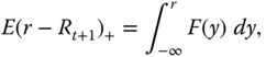
Figure 10.9 shows a level set ![]() with blue color. The blue and red regions together show the domain of the function
with blue color. The blue and red regions together show the domain of the function ![]() . In panel (a) function
. In panel (a) function ![]() is calculated from the monthly returns of of S&P 500. In panel (b) the returns are of US Treasury 10-year bond. The level
is calculated from the monthly returns of of S&P 500. In panel (b) the returns are of US Treasury 10-year bond. The level ![]() is the Sharpe ratio over the complete period. Parameter
is the Sharpe ratio over the complete period. Parameter ![]() in the definition of the domain of
in the definition of the domain of ![]() is equal to 36 months. Thus, the blue region shows the time periods
is equal to 36 months. Thus, the blue region shows the time periods ![]() for which the Sharpe ratio is above the usual value, and the red region shows the time periods
for which the Sharpe ratio is above the usual value, and the red region shows the time periods ![]() for which the Sharpe ratio is below the usual value.
for which the Sharpe ratio is below the usual value.
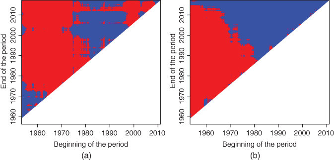
Figure 10.9 Sharpe ratios for every period: Level sets. We show a level set  in (10.39) with blue color. (a) Function
  is the Sharpe ratio of S&P 500; (b) function
  is the Sharpe ratio of US Treasury 10-year bond. The blue regions show the time periods
  for which the Sharpe ratio is above the usual value, and the red color shows when it is below the usual value.
10.5.2.2 Sharpe Ratios Over a Sequence of Intervals
A useful way to visualize function ![]() , defined in (10.36), is to draw slices of this function. Slices are univariate functions
, defined in (10.36), is to draw slices of this function. Slices are univariate functions
where ![]() and
and ![]() are fixed. When
are fixed. When ![]() is fixed, then we are looking at Sharpe ratios over periods with a fixed starting point
is fixed, then we are looking at Sharpe ratios over periods with a fixed starting point ![]() . When
. When ![]() is fixed, then we are looking at Sharpe ratios over periods with a fixed end point
is fixed, then we are looking at Sharpe ratios over periods with a fixed end point ![]() . For function
. For function ![]() we choose
we choose ![]() so that
so that ![]() , and then
, and then ![]() satisfies
satisfies ![]() . For function
. For function ![]() we choose
we choose ![]() so that
so that ![]() , and then
, and then ![]() satisfies
satisfies ![]() .
.
Figure 10.10 shows slices of function ![]() . Panel (a) shows slices
. Panel (a) shows slices ![]() , where
, where ![]() (red),
(red), ![]() (blue),
(blue), ![]() (green), and
(green), and ![]() (black). Panel (b) shows slices
(black). Panel (b) shows slices ![]() , where
, where ![]() (black),
(black), ![]() (red),
(red), ![]() (blue), and
(blue), and ![]() (green).
(green).
Figure 10.10 Time series of Sharpe ratios: Slices. (a) A slice at time  shows the Sharpe ratio computed with the data starting at
  and ending
  , where
  (red),
  (blue),
  (green), and
  (black). (b) A slice at time
  shows the Sharpe ratio computed with the data starting at
  and ending
  , where
  (black),
  (red),
  (blue), and
  (green).
Figure 10.11 shows function ![]() as black curves. In panel (a) we use S&P 500 monthly returns and in panel (b) we use monthly returns of US Treasury 10-year bond. Parameter
as black curves. In panel (a) we use S&P 500 monthly returns and in panel (b) we use monthly returns of US Treasury 10-year bond. Parameter ![]() is equal to 120 months. The green curves show time series of means:
is equal to 120 months. The green curves show time series of means: ![]() , and the blue curves show time series of standard deviations:
, and the blue curves show time series of standard deviations: ![]() , where
, where ![]() is defined in (10.37) and
is defined in (10.37) and ![]() is defined in (10.38). Note that the upper borders of the level sets in Figure 10.9 show the level sets of black functions in Figure 10.11. The violet horizontal lines show the Sharpe ratios over the complete time period.
is defined in (10.38). Note that the upper borders of the level sets in Figure 10.9 show the level sets of black functions in Figure 10.11. The violet horizontal lines show the Sharpe ratios over the complete time period.
Both time series of Sharpe ratios of S&P 500 and 10-year bond show a similar pattern: The Sharpe ratios make a jump at the end of 1970s. This pattern is more profound for 10-year bond than for S&P 500. We can see that the changes in the time series of Sharpe ratios are caused mainly by the changes in the time series of the arithmetic means of the returns.

Figure 10.11 Time series of Sharpe ratios. (a) Sharpe ratios of S&P 500; (b) Sharpe ratios of US 10-year bond. The black curves show the Sharpe ratios, the green curves show the means of the excess returns, and the blue curves show the standard deviations of the excess returns. The time series at time  show Sharpe ratios computed with the data starting at
  and ending
  . The violet horizontal lines show the Sharpe ratios over the complete time period.
Note that the Sharpe ratios in Figure 10.11 are relevant in the case when we choose time point ![]() to divide the historical data to the estimation part and to the testing part. After that we calculate the Sharpe ratio from the historically simulated returns
to divide the historical data to the estimation part and to the testing part. After that we calculate the Sharpe ratio from the historically simulated returns ![]() , and compare the Sharpe ratio to the Sharpe ratio of a benchmark (S&P 500 or 10-year bond). The choice of time point
, and compare the Sharpe ratio to the Sharpe ratio of a benchmark (S&P 500 or 10-year bond). The choice of time point ![]() affects the Sharpe ratio of the benchmark, as shown by the black curve in Figure 10.11, and in a sense, we study the robustness of the performance measures of the benchmarks to the choice of the time point
affects the Sharpe ratio of the benchmark, as shown by the black curve in Figure 10.11, and in a sense, we study the robustness of the performance measures of the benchmarks to the choice of the time point ![]() , which sets the beginning of the testing period.
, which sets the beginning of the testing period.
10.5.3 Using the Certainty Equivalent in Evaluation
The certainty equivalent can be used in much the same way as the Sharpe ratio. Sample certainty equivalent is defined in (10.13). Given a time series ![]() of gross returns, we define the sample certainty equivalent over interval
of gross returns, we define the sample certainty equivalent over interval ![]() as
as

where ![]() is a utility function. Parameter
is a utility function. Parameter ![]() guarantees that there are at least two observations to calculate the certainty equivalent. The slices of function
guarantees that there are at least two observations to calculate the certainty equivalent. The slices of function ![]() are often more informative than contour plots or perspective plots. Slices are univariate functions
are often more informative than contour plots or perspective plots. Slices are univariate functions
where ![]() and
and ![]() are fixed. For function
are fixed. For function ![]() we choose
we choose ![]() so that
so that ![]() , and then
, and then ![]() satisfies
satisfies ![]() . For function
. For function ![]() we choose
we choose ![]() so that
so that ![]() , and then
, and then ![]() satisfies
satisfies ![]() .
.

Figure 10.12 Time series of certainty equivalents. (a) Certainty equivalents of S&P 500; (b) certainty equivalents of US Treasury 10-year bond. The green curves show the case of risk aversion  , the red curves have
  , and the purple curves have
  . Time series at time
  show certainty equivalents computed with the data starting at
  and ending
  .
.
Figure 10.12 shows function ![]() : the sample mean is taken only over the last part of the original return time series. We have chosen
: the sample mean is taken only over the last part of the original return time series. We have chosen ![]() . In panel (a) the returns
. In panel (a) the returns ![]() are monthly gross returns of S&P 500 index, and in panel (b) the returns
are monthly gross returns of S&P 500 index, and in panel (b) the returns ![]() are monthly gross returns of US Treasury 10-year bond. The utility function
are monthly gross returns of US Treasury 10-year bond. The utility function ![]() is the power utility function, defined in (9.28). The green curve shows certainty equivalents when the risk aversion parameter of the utility function is
is the power utility function, defined in (9.28). The green curve shows certainty equivalents when the risk aversion parameter of the utility function is ![]() (plain gross returns), the red curve shows the case
(plain gross returns), the red curve shows the case ![]() (logarithmic utility), and the purple curve shows the case
(logarithmic utility), and the purple curve shows the case ![]() . Note that the green curves in Figure 10.11 show the means of the excess returns, whereas the green curves in Figure 10.12 show the means of the gross returns.
. Note that the green curves in Figure 10.11 show the means of the excess returns, whereas the green curves in Figure 10.12 show the means of the gross returns.
We can see that the certainty equivalents of S&P 500 are rather stable when the testing period starts before the mid-1990s, whereas the certainty equivalents of 10-year bond are rather unstable even when the testing period starts early. The risk aversion parameter ![]() does not change qualitatively time series but affects only the level: a lower risk aversion leads to a larger certainty equivalent.
does not change qualitatively time series but affects only the level: a lower risk aversion leads to a larger certainty equivalent.
Derivation of this with respect to ![]() , and setting the gradient to zero, gives the equations
, and setting the gradient to zero, gives the equations
which leads to the solution (10.32).

where ![]() is the return of a market index,
is the return of a market index, ![]() is the return of the risk-free rate,
is the return of the risk-free rate,  , and
, and ![]() .
.

and

Note that the sample Sharpe ratio is defined in (10.3).