
Chapter 11
Markowitz Portfolios
Portfolio choice with mean–variance preferences was proposed by Markowitz (1952 1959). The approach introduced the idea of balancing risk and return to find an optimal portfolio.
Markowitz approach can be used in the single period portfolio selection. Let ![]() be the portfolio return. In the Markowitz approach there exists three ways to choose the portfolio:
be the portfolio return. In the Markowitz approach there exists three ways to choose the portfolio:
- 1. Maximize the variance penalized expected return

- where
 is the risk aversion coefficient. Parameter
  measures the investor's relative risk aversion, as defined in (9.31).
 - 2. Minimize the variance
 under a minimal requirement for the expected return:
  , where
  is the minimal requirement for the expected return.
 - 3. Maximize the expected return
 under a condition that the variance is not too large:
  where
where  is the largest allowed standard deviation for the return.
Here ![]() and
and ![]() mean the conditional expectation and the conditional variance, conditional on the information available at time
mean the conditional expectation and the conditional variance, conditional on the information available at time ![]() .
.
The variance penalized expected return was already discussed in Section 9.2.1. The variance penalized expected return is convenient because it involves explicitly the risk aversion parameter ![]() , which makes it possible to find a connection to the maximization of an expected utility. The other two approaches involve risk aversion more implicitly. When variance is minimized under a minimal requirement
, which makes it possible to find a connection to the maximization of an expected utility. The other two approaches involve risk aversion more implicitly. When variance is minimized under a minimal requirement ![]() for the expected return, then the minimal requirement
for the expected return, then the minimal requirement ![]() is a risk aversion parameter, because smaller values of
is a risk aversion parameter, because smaller values of ![]() are associated with more risk aversion. When the expected return is maximized under a condition that the variance is less than or equal to
are associated with more risk aversion. When the expected return is maximized under a condition that the variance is less than or equal to ![]() , then
, then ![]() is a risk aversion parameter, because smaller values of
is a risk aversion parameter, because smaller values of ![]() indicate more risk aversion.
indicate more risk aversion.
We explain with the help of Markowitz bullets the concepts of the minimum variance portfolio, the tangency portfolio, and the efficient frontier. This is done in Section 11.3.
The method of Lagrange multipliers appears in Section 11.1.2 and in Section 11.2. The method of Lagrange multipliers is a useful general method of optimization. The method of Lagrange multipliers helps to cope with the restriction that the sum of portfolio weights have to be equal to one. Further complications appear when we want to restrict ourselves to long-only portfolios, or to make some other additional restrictions on the portfolio weights. We do not consider these additional complications.
We use the notations of Section 9.1. The portfolio return was defined in (9.3) as

where
is the vector of the portfolio weights, ![]() is the transpose of the column vector
is the transpose of the column vector ![]() , and
, and
is the vector of the gross returns of the portfolio components. The portfolio weights satisfy the constraint

Thus, ![]() and
and
where ![]() is called the excess return. Since we consider only single period portfolio selection, we do not need the time subscript in the notation. Thus, we denote the portfolio vector of risky assets by
is called the excess return. Since we consider only single period portfolio selection, we do not need the time subscript in the notation. Thus, we denote the portfolio vector of risky assets by
Also, since the expectations and variances are conditional on ![]() , the risk-free rate is a constant (known at time
, the risk-free rate is a constant (known at time ![]() ). We will denote the risk-free rate by
). We will denote the risk-free rate by
The vector of means and the covariance matrix of the risky assets is denoted by
where ![]() and
and ![]() is the
is the ![]() matrix with elements
matrix with elements ![]() . Now,
. Now,
Section 11.1 considers the maximization of the variance penalized expected return. Section 11.2 considers minimization of the variance under a minimal requirement for the expected return. Section 11.3 considers concepts related to the Markowitz portfolio theory, such as the minimum variance portfolio and the tangency portfolio. Section 11.4 considers further topics related to Markowitz portfolio theory. Section 11.5 applies Markowitz formulas to portfolio selection.
11.1 Variance Penalized Expected Return
We consider the maximization of the variance penalized expected return. Section 11.1.1 considers portfolios where the risk-free rate is included. Section 11.1.2 considers portfolios without the risk-free rate.
11.1.1 Variance Penalization with the Risk-Free Rate
Let us consider the maximization of the variance penalized expected return when the risk-free rate is included. We consider first the general case of ![]() risky asset and then the special cases of one risky asset and two risky assets.
risky asset and then the special cases of one risky asset and two risky assets.
11.1.1.1 Several Risky Assets and the Risk-Free Rate
The portfolio components are ![]() risky assets and the risk-free rate. Let the return of the risk-free investment be
risky assets and the risk-free rate. Let the return of the risk-free investment be ![]() . We allocate the proportion
. We allocate the proportion ![]() into the risk-free investment. Then the portfolio return is
into the risk-free investment. Then the portfolio return is
We choose the weight vector ![]() as maximizing
as maximizing
Derivating with respect to ![]() and setting the partial derivatives to zero gives
and setting the partial derivatives to zero gives
Thus,
11.1.1.2 One Risky Asset and the Risk-Free Rate
Let us invest the proportion ![]() to a stock and
to a stock and ![]() to the risk-free rate whose gross return is
to the risk-free rate whose gross return is ![]() . Now the gross return of the portfolio is
. Now the gross return of the portfolio is
where ![]() is the return of the stock. Let the expected return of the stock be
is the return of the stock. Let the expected return of the stock be ![]() and the variance
and the variance ![]() . Then,
. Then,
Setting the derivative with respect to ![]() to zero and solving for
to zero and solving for ![]() gives the maximizer of (11.2) as
gives the maximizer of (11.2) as
Let ![]() be the optimal weight of the long-only portfolio. The maximizer
be the optimal weight of the long-only portfolio. The maximizer ![]() of (11.2) under the restriction that
of (11.2) under the restriction that ![]() is obtained by projecting the unrestricted solution on
is obtained by projecting the unrestricted solution on ![]() . Thus,
. Thus,

where ![]() is given in (11.3).
is given in (11.3).
11.1.1.3 Two Risky Assets and the Risk-Free Rate
Let us have two stocks and the risk-free rate and let us invest the proportion ![]() in the first stock, proportion
in the first stock, proportion ![]() in the second stock, and proportion
in the second stock, and proportion ![]() in the risk-free rate. Now the portfolio return is
in the risk-free rate. Now the portfolio return is
where ![]() is the return of the first stock and
is the return of the first stock and ![]() is the return of the second stock. Let the expected returns of the stocks be
is the return of the second stock. Let the expected returns of the stocks be ![]() ,
, ![]() and let the variances of the returns be
and let the variances of the returns be ![]() ,
, ![]() . Denote the covariance of the returns by
. Denote the covariance of the returns by ![]() . We have
. We have

Setting derivatives with respect to ![]() and
and ![]() to zero gives
to zero gives

Thus,1

and

11.1.2 Variance Penalization without the Risk-Free Rate
Let us consider the maximization of the variance penalized expected return when the risk-free rate is excluded. We solve first the case of ![]() risky assets and then the case of two risky assets.
risky assets and then the case of two risky assets.
11.1.2.1 Several Risky Assets
The maximization of the variance penalized expected return chooses the weight vector ![]() as maximizing
as maximizing
where ![]() is the vector of length
is the vector of length ![]() whose all elements are equal to one, so that the constraint is
whose all elements are equal to one, so that the constraint is

Let us maximize
under the constraint ![]() . We use the method of Lagrange multipliers and maximize the Lagrange function
. We use the method of Lagrange multipliers and maximize the Lagrange function
where ![]() is the Lagrange multiplier. Derivating with respect to
is the Lagrange multiplier. Derivating with respect to ![]() and
and ![]() and setting the partial derivatives to zero we get
and setting the partial derivatives to zero we get

Thus,
Let us solve ![]() from
from ![]() , which leads to
, which leads to
and finally

11.1.2.2 Two Risky Assets
Let us have two stocks and put the proportion ![]() to the first stock and proportion
to the first stock and proportion ![]() to the second stock. Now,
to the second stock. Now,
Let the expected returns of the stocks be ![]() ,
, ![]() and let the variances of the returns be
and let the variances of the returns be ![]() ,
, ![]() . Denote the covariance of the returns by
. Denote the covariance of the returns by ![]() . We have
. We have

Setting the derivative with respect to ![]() to zero and solving for
to zero and solving for ![]() gives
gives

Note that the maximizer ![]() under the restriction that
under the restriction that ![]() is obtained by projecting the unrestricted solution:
is obtained by projecting the unrestricted solution:
where ![]() is given in (11.6).
is given in (11.6).
11.2 Minimizing Variance under a Sufficient Expected Return
We consider the minimization of the variance under a condition that the expected return should be sufficiently large. Section 11.2.1 considers portfolios where the risk-free rate is included. Section 11.2.2 considers portfolios without the risk-free rate.
11.2.1 Minimizing Variance with the Risk-Free Rate
We consider first the case of ![]() risky assets and the risk-free investment, and then the case of one risky assets and the risk-free investment.
risky assets and the risk-free investment, and then the case of one risky assets and the risk-free investment.
11.2.1.1 Several Risky Assets and the Risk-Free Rate
Let us consider the case of ![]() risky assets and a risk-free investment. We want to find the weight vector minimizing
risky assets and a risk-free investment. We want to find the weight vector minimizing
where ![]() . We should choose
. We should choose ![]() , so that the required expected return is not smaller than the risk-free return.
, so that the required expected return is not smaller than the risk-free return.
The return vector of the risky investments is denoted by ![]() , the expectation vector is
, the expectation vector is ![]() , the covariance matrix is
, the covariance matrix is ![]() , and the risk-free return is
, and the risk-free return is ![]() . The proportion
. The proportion ![]() is invested in the risk-free asset. The return of the portfolio is
is invested in the risk-free asset. The return of the portfolio is
The expected return of the portfolio is
Let us find ![]() minimizing
minimizing
under the constraint
where ![]() is a constant. Define the Lagrange function
is a constant. Define the Lagrange function
where ![]() is the Lagrange multiplier. We solve the equation
is the Lagrange multiplier. We solve the equation
to get
The constraint can be written as
which implies
and
Thus, the vector of the weights of the risky investments is
11.2.1.2 One Risky Asset and the Risk-Free Rate
Let us consider the case where we have one risky asset with return ![]() and a risk-free investment with return
and a risk-free investment with return ![]() . Let the expected return of the risky asset be
. Let the expected return of the risky asset be ![]() and the variance
and the variance ![]() . Let us invest the proportion
. Let us invest the proportion ![]() to the risky asset and the proportion
to the risky asset and the proportion ![]() to the risk-free asset. The return of the portfolio is
to the risk-free asset. The return of the portfolio is
The expected return of the portfolio is
and the variance of the portfolio is
We want that the expected return should be at least ![]() and we minimize the variance under this condition. Thus, we want to find
and we minimize the variance under this condition. Thus, we want to find ![]() minimizing
minimizing
under the constraint
Define the Lagrange function
where ![]() is the Lagrange multiplier. The solution of the equation
is the Lagrange multiplier. The solution of the equation
is
The constraint ![]() implies
implies ![]() Thus, the weight of the risky investment is
Thus, the weight of the risky investment is
When ![]() , then
, then ![]() .
.
11.2.2 Minimizing Variance without the Risk-Free Rate
We want to choose the weight vector ![]() minimizing
minimizing
where ![]() , and we should choose
, and we should choose ![]() , so that the required expected return is not smaller than the risk-free return.
, so that the required expected return is not smaller than the risk-free return.
Let us consider portfolios of ![]() risky assets and exclude the risk-free investment. The return vector of the risky investments is denoted by
risky assets and exclude the risk-free investment. The return vector of the risky investments is denoted by ![]() . Let us denote
. Let us denote ![]() and
and ![]() . Then,
. Then,
We minimize
under the constraints
where ![]() is the column vector of length
is the column vector of length ![]() whose elements are equal to 1, and
whose elements are equal to 1, and ![]() is a constant. The Lagrange function is
is a constant. The Lagrange function is
where ![]() are the Lagrange multipliers. The solution of the equation2
are the Lagrange multipliers. The solution of the equation2
is
To get ![]() and
and ![]() we need to solve the equations
we need to solve the equations

Denoting ![]() ,
, ![]() , and
, and ![]() , we get
, we get

Then, the vector of the portfolio weights is
where ![]() .
.
11.3 Markowitz Bullets
A Markowitz bullet is a scatter plot of points, where each point corresponds to a portfolio, the ![]() -coordinate of a point is the standard deviation of the return of the portfolio, and the
-coordinate of a point is the standard deviation of the return of the portfolio, and the ![]() -coordinate of a point is the expected return of the portfolio. The scatter plot is called a bullet because the boundary of the scatter plot is a part of a hyperbola, and thus its shape resembles the shape of a bullet.3
-coordinate of a point is the expected return of the portfolio. The scatter plot is called a bullet because the boundary of the scatter plot is a part of a hyperbola, and thus its shape resembles the shape of a bullet.3
Figure 11.1 plots a collection of portfolios which are obtained from two risky assets. The expected net returns of the assets are 1 and 0.5. The standard deviations are 2 and 1. The correlation between the returns of the risky assets varies from ![]() to 1. Panel (a) shows long-only portfolios. The blue wedge on the left shows all portfolios that can be obtained when correlation is
to 1. Panel (a) shows long-only portfolios. The blue wedge on the left shows all portfolios that can be obtained when correlation is ![]() . The orange vector on the right shows all portfolios that can be obtained when correlation is 1. When correlation is
. The orange vector on the right shows all portfolios that can be obtained when correlation is 1. When correlation is ![]() , then there exists a portfolio with zero variance. The portfolio with zero variance should have the same return as the risk-free rate, to exclude arbitrage. Panel (b) shows portfolios that can be obtained from the two risky assets when shorting is allowed. The weight of an asset varies between
, then there exists a portfolio with zero variance. The portfolio with zero variance should have the same return as the risk-free rate, to exclude arbitrage. Panel (b) shows portfolios that can be obtained from the two risky assets when shorting is allowed. The weight of an asset varies between ![]() and 1.5.
and 1.5.

Figure 11.1 Markowitz bullets: Portfolios of two risky assets when correlation varies. (a) Shown are long-only portfolios that can be obtained from two risky assets when correlation between the risky assets varies between  and
and  . (b) Shorting is allowed.
Figure 11.2 shows portfolios obtained from three risky assets as a blue area. The three risky assets are shown as orange points. The correlations between the risky assets are 0.2, 0.5, and 0.6. Panel (a) shows all long-only portfolios and panel (b) shows portfolios when shorting is allowed with restrictions. The shapes of the blue areas are irregular but the left boundaries are parts of hyperbolas.

Figure 11.2 Markowitz bullets: Portfolios of three risky assets. (a) Long-only portfolios that can be obtained from three risky assets. (b) Portfolios when shorting is allowed.
Figure 11.3 shows a Markowitz bullet of long-only portfolios, when the risk-free rate is included and the borrowing is allowed. Panel (a) shows as a blue curve long-only portfolios whose components are two risky assets with correlation ![]() . The green point shows the minimum variance portfolio. The black point shows the risk-free investment whose net return is 0.1 and the variance is zero. The red point shows the tangency portfolio. The red line joining the risk-free investment and the tangency portfolio corresponds to the long-only portfolios whose components are the risk-free investment and the tangency portfolio. The yellow area corresponds to the long-only portfolios whose components are the risk-free investment and one of the portfolios on the blue curve; these are all possible long-only portfolios. Panel (b) shows portfolios from two risky assets and the risk-free investment when the weight of the risk-free investment is allowed to be negative, which amounts to allowing leveraging by borrowing.
. The green point shows the minimum variance portfolio. The black point shows the risk-free investment whose net return is 0.1 and the variance is zero. The red point shows the tangency portfolio. The red line joining the risk-free investment and the tangency portfolio corresponds to the long-only portfolios whose components are the risk-free investment and the tangency portfolio. The yellow area corresponds to the long-only portfolios whose components are the risk-free investment and one of the portfolios on the blue curve; these are all possible long-only portfolios. Panel (b) shows portfolios from two risky assets and the risk-free investment when the weight of the risk-free investment is allowed to be negative, which amounts to allowing leveraging by borrowing.

Figure 11.3 Markowitz bullet: Long-only portfolios and leveraging. Panel (a) shows long-only portfolios for two risky assets and the risk-free investment. Panel (b) shows portfolios for two risky assets and the risk-free investment when the weight of the risk-free investment is allowed to be negative, which means the borrowing is allowed.
We can use Figure 11.3 to define the concepts of the minimum variance portfolio, the tangency portfolio, and the efficient frontier.
- 1. The minimum variance portfolio is the portfolio of risky assets whose variance is the smallest among all portfolios of risky assets. When the risk-free rate is included, then the risk-free investment has the minimum variance zero.
- 2. Efficient frontier is the collection of those portfolio vectors that have the expected return greater than or equal to the expected return of the minimum variance portfolio:
In Figure 11.3(a) the efficient frontier without the risk-free rate is the part of the blue curve going upward from the red point, but when the risk-free rate is included, then the red vector from the risk-free asset to the tangency portfolio, followed by the blue curve shows the efficient frontier. The efficient frontier consists of possible portfolios a rational investor should consider, because these portfolios have a higher expected return with the same variance than other portfolios. Adding the risk-free rate gives the possibility to get portfolios with a smaller standard deviation than any of the pure stock portfolios: some of the portfolios on the red vector are such that the standard error is smaller than the standard deviation of any of the pure stock portfolios.
In Figure 11.3(b) borrowing is allowed. The borrowed money is invested in the stocks. Now the efficient frontier is the red half line starting from the risk-free investment and passing the tangency portfolio. We see that a rational investor chooses only portfolios that are a combination of the risk-free investment and the tangency portfolio. The other portfolios have a smaller expected return for the same variance.
- 3. The tangency portfolio is a portfolio which has the largest Sharpe ratio. Indeed, the tangency portfolio maximizes the slope of the vector drawn from the risk-free asset to a pure stock portfolio. The slope of the vector from the point
 to the point
 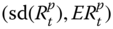 is equal to the Sharpe ratio
  , where
  is the return of the risk-free asset and
  is the return of a portfolio.
 - 4. It can be argued that the tangency portfolio, shown as the red point in the blue curve, is in fact the market portfolio, because the rational investor buys only a combination of the tangency portfolio and the risk-free asset, and thus the price of the tangency portfolio is in the equilibrium equal to the price of the market portfolio.
Figure 11.4 plots standard deviations and means for a collection of portfolios when shorting of a stock is allowed. Panel (a) shows portfolios from two risky assets. The blue part shows the long-only portfolios, the orange part shows the portfolios where the less risky stock is shorted, and the purple part shows the portfolios where the more risky stock is shorted. The green bullet shows the minimum variance portfolio, the black bullet shows the risk-free investment, and the red bullet shows the tangency portfolio. Panel (b) shows portfolios of two risky assets and a risk-free investment when the weight of the risk-free investment is allowed to be negative, which amounts to allowing leveraging by borrowing.
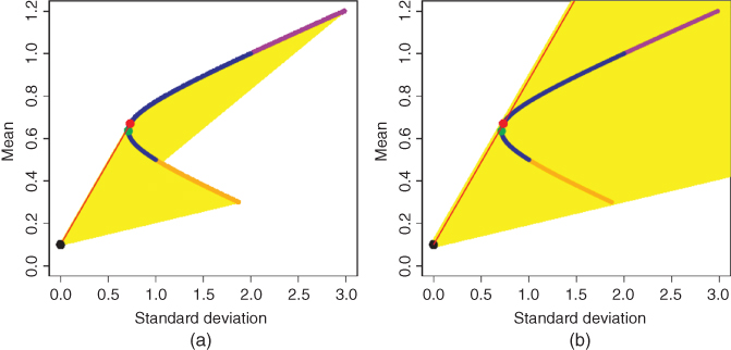
Figure 11.4 Markowitz bullet: Shorting and leveraging. Panel (a) shows portfolios from two risky assets, and from two risky assets and the risk-free investment. Panel (b) shows portfolios from two risky assets and a risk-free investment when the weight of the risk-free investment is allowed to be negative, so that borrowing is possible.
Figure 11.5 shows how increasing the number of basis assets makes the Markowitz bullet larger. The blue hyperbola shows portfolios that can be obtained from two risky assets, the green area shows portfolios that can be obtained from three risky assets, and the yellow area shows portfolios that can be obtained from four risky assets. The orange points show the risky assets. The covariances between the returns of the risky assets are zero.

Figure 11.5 Markowitz bullet: Uncorrelated assets. Markowitz bullets are shown for an increasing number of assets: blue curve shows portfolios from two risky assets, the green area portfolios from three risky assets, and the yellow area portfolios from four risky assets, when the risky assets are uncorrelated.
Figure 11.6 studies a Markowitz bullet of the daily returns of S&P 500 components. The data is described in Section 2.4.5. Panel (a) shows a scatter plot of the annualized sample standard deviations and annualized sample means of the excess returns of the stocks included in the S&P 500 components data. The red bullet shows the location of the S&P 500 index. The blue bullet is at the origin: we take the risk-free rate equal to zero because the Markowitz bullet is computed from the excess returns.4 Panel (b) shows a kernel density estimate of the distribution of the Sharpe ratios of the stocks included in S&P 500 components data. The red vertical line indicates the Sharpe ratio of the S&P 500 index. We see that the S&P 500 is not a tangent portfolio, since its Sharpe ratio is smaller than the most Sharpe ratios of the individual stocks.

Figure 11.6 Markowitz bullet: S&P 500 components. (a) A scatter plot of annualized sample standard deviations and means of excess returns of a collection of stocks in the S&P 500 index. (b) A kernel density estimate of the distribution of the Sharpe ratios.
11.4 Further Topics in Markowitz Portfolio Selection
11.4.1 Estimation
In order to apply Markowitz formulas, we have to estimate the vector ![]() of expected returns and the covariance matrix
of expected returns and the covariance matrix ![]() of the returns of the risky assets.
of the returns of the risky assets.
The sample means, sample variances, and sample covariances could be applied. However, we have discussed many other methods. Chapter 6 discusses various prediction methods that could be applied to estimate (predict) ![]() . Chapter 7 discusses various methods for volatility prediction that could be used to estimate
. Chapter 7 discusses various methods for volatility prediction that could be used to estimate ![]() ,
, ![]() . Analogous methods can be used to estimate the covariances
. Analogous methods can be used to estimate the covariances ![]() ,
, ![]() ,
, ![]() . For example, Section 5.4 considers multivariate time series models which are relevant for covariance prediction.
. For example, Section 5.4 considers multivariate time series models which are relevant for covariance prediction.
In the estimation of the covariance matrix ![]() we have to take the curse of dimensionality into account, since the number
we have to take the curse of dimensionality into account, since the number ![]() of risky assets can be high relative to the sample size. Note that the covariance matrix involves only the pairwise covariances, so that high dimensionality does not make it difficult to estimate any single component of the matrix
of risky assets can be high relative to the sample size. Note that the covariance matrix involves only the pairwise covariances, so that high dimensionality does not make it difficult to estimate any single component of the matrix ![]() . However, there are
. However, there are ![]() covariances, and a simultaneous estimation of such a large number of parameters is difficult.
covariances, and a simultaneous estimation of such a large number of parameters is difficult.
11.4.2 Penalizing Techniques
Let us consider minimization of the variance of the portfolio return under a minimal requirement for the expected return. Let ![]() be the return vector of risky assets with
be the return vector of risky assets with ![]() and
and ![]() . Then the expected return of the portfolio is
. Then the expected return of the portfolio is ![]() and the variance is
and the variance is ![]() , where
, where ![]() is the vector of portfolio weights. We want to find weights
is the vector of portfolio weights. We want to find weights ![]() such that
such that
is minimized under the constraints
where ![]() is the requirement for the expected return of the portfolio. The minimization problem is equivalent to finding
is the requirement for the expected return of the portfolio. The minimization problem is equivalent to finding ![]() such that
such that
is minimized under the same constraints. Let us assume to have observed historical returns ![]() of the basis assets. The empirical version of the minimization problem is to find
of the basis assets. The empirical version of the minimization problem is to find ![]() such that
such that

is minimized under the constraints
where ![]() . Brodie et al. (2009) proposed to add a penalization term and find
. Brodie et al. (2009) proposed to add a penalization term and find ![]() minimizing
minimizing

under the same constraints, where ![]() is the regularizing parameter. The approach is similar to the approach in Lasso regression of Tibshirani (1996).
is the regularizing parameter. The approach is similar to the approach in Lasso regression of Tibshirani (1996).
DeMiguel et al. (2009) showed that it is difficult to significantly or consistently outperform the naive strategy in which each available asset is given an equal weight in the portfolio.
11.4.3 Principal Components Analysis
Let ![]() be the
be the ![]() vector of the expected returns of the
vector of the expected returns of the ![]() risky assets. Given the
risky assets. Given the ![]() vector of portfolio weights
vector of portfolio weights ![]() , the return of the portfolio is
, the return of the portfolio is ![]() . Let
. Let ![]() be the
be the ![]() covariance matrix of the returns of the risky assets. We can make the principal component analysis of the covariance matrix and write
covariance matrix of the returns of the risky assets. We can make the principal component analysis of the covariance matrix and write
where ![]() is the
is the ![]() matrix whose columns are the eigenvectors of
matrix whose columns are the eigenvectors of ![]() and
and ![]() is the
is the ![]() diagonal matrix, whose diagonal elements are the eigenvalues of
diagonal matrix, whose diagonal elements are the eigenvalues of ![]() . We get
. We get ![]() uncorrelated principal portfolios whose return vector is
uncorrelated principal portfolios whose return vector is ![]() . We can think of these principal portfolios as new basic assets and write any portfolio in terms of the principal components. If the original weights are
. We can think of these principal portfolios as new basic assets and write any portfolio in terms of the principal components. If the original weights are ![]() , then the new weights are
, then the new weights are ![]() . Now we can calculate the variance of the portfolio as
. Now we can calculate the variance of the portfolio as

where ![]() are the eigenvalues of
are the eigenvalues of ![]() . We can define the diversification distribution
. We can define the diversification distribution

where ![]() . We can say that a portfolio is better diversified, if the diversification distribution is closer to the uniform distribution. This can be measured by
. We can say that a portfolio is better diversified, if the diversification distribution is closer to the uniform distribution. This can be measured by

Partovi and Caputo (2004) used principal portfolios in their discussion of efficient frontier, and Meucci (2009) presented the idea of the diversification distribution.
11.5 Examples of Markowitz Portfolio Selection
We illustrate Markowitz portfolio selection using as the basic assets the S&P 500 and Nasdaq-100 indexes. The daily data set of S&P 500 and Nasdaq-100 is described in Section 2.4.2.
We consider portfolio selection without the risk-free rate. We maximize the variance penalized expected return (11.5) both without restrictions and with the restriction to the long-only weights.
Figure 11.7 shows the time series of the Markowitz weights of S&P 500. Panel (a) shows the unrestricted Markowitz weights and panel (b) shows the long-only Markowitz weights. The risk aversion parameter takes values ![]() (black, red, blue, green, and orange). When the weight of S&P 500 is denoted by
(black, red, blue, green, and orange). When the weight of S&P 500 is denoted by ![]() , then the weight of Nasdaq-100 is
, then the weight of Nasdaq-100 is ![]() . We have estimated the mean vector and the covariance matrix sequentially, using the sample means and the sample covariance matrices. We start when there are 1000 observations (4 years of data). The weight of S&P 500 increases when the risk aversion parameter
. We have estimated the mean vector and the covariance matrix sequentially, using the sample means and the sample covariance matrices. We start when there are 1000 observations (4 years of data). The weight of S&P 500 increases when the risk aversion parameter ![]() increases. After year 2000, the weight of S&P 500 jumps higher.
increases. After year 2000, the weight of S&P 500 jumps higher.

Figure 11.7 S&P 500 and Nasdaq-100: Markowitz weights. The time series of the weights for the S&P 500. (a) The unrestricted weights and (b) the long-only weights. The risk aversion parameter takes values  (black, red, blue, green, and orange).
Figure 11.8 shows the Sharpe ratios, annualized means and annualized standard deviations, as a function of risk aversion parameter ![]() . Panel (a) shows the Sharpe ratios. The black line with labels “1” is obtained when the unrestricted weights are used and the green line with labels “2” is obtained when the long-only weights are used. The horizontal lines show the Sharpe ratios for S&P 500 (blue) and Nasdaq-100 (red). The risk-free rate is deduced from the 1-month US bill rates, described in Section 2.4.3. The highest value of the Sharpe ratio is obtained for small risk aversion. When the risk aversion increases, the Sharpe ratios of the Markowitz portfolio approach the Sharpe ratio of S&P 500. Panel (b) shows the annualized means as a function of the risk aversion and panel (c) shows the annualized standard deviations. Both means and standard deviations increase sharply when the risk aversion parameter decreases.
. Panel (a) shows the Sharpe ratios. The black line with labels “1” is obtained when the unrestricted weights are used and the green line with labels “2” is obtained when the long-only weights are used. The horizontal lines show the Sharpe ratios for S&P 500 (blue) and Nasdaq-100 (red). The risk-free rate is deduced from the 1-month US bill rates, described in Section 2.4.3. The highest value of the Sharpe ratio is obtained for small risk aversion. When the risk aversion increases, the Sharpe ratios of the Markowitz portfolio approach the Sharpe ratio of S&P 500. Panel (b) shows the annualized means as a function of the risk aversion and panel (c) shows the annualized standard deviations. Both means and standard deviations increase sharply when the risk aversion parameter decreases.

Figure 11.8 S&P 500 and Nasdaq-100: Sharpe ratios, means, and standard deviations. (a) The Sharpe ratios as a function of  ; (b) the annualized means; (c) the annualized standard deviations. The black line with labels “1” is obtained when the unrestricted weights are used and the green line with labels “2” is obtained when the long-only weights are used.

This leads to
