
Chapter 5
Time Series Analysis
Time series analysis can be used to analyze both a univariate time series and a vector time series. We are interested in estimating the dependence between consecutive observations. In a vector time series there is both cross-sectional dependence and time series dependence, which means that the components of the vector depend on each other at any given point of time, and the future values of the vectors depend on the past values of the vectors.
Model free time series analysis can estimate the joint distribution of
for some ![]() . The estimation could be done using nonparametric multivariate density estimation. A different model free approach models at the first step the distribution of
. The estimation could be done using nonparametric multivariate density estimation. A different model free approach models at the first step the distribution of ![]() parametrically, using density
parametrically, using density ![]() . At the second step, parameter
. At the second step, parameter ![]() is taken to be time dependent. This leads to a semiparametric time series analysis, because we combine a cross-sectional parametric model with a time varying estimation of the parameter. Time localized maximum likelihood or time localized least squares can be used to estimate the parameter. Of particular interest is to estimate a univariate excess distribution
is taken to be time dependent. This leads to a semiparametric time series analysis, because we combine a cross-sectional parametric model with a time varying estimation of the parameter. Time localized maximum likelihood or time localized least squares can be used to estimate the parameter. Of particular interest is to estimate a univariate excess distribution ![]() with a time varying
with a time varying ![]() , because this leads to time varying quantile estimation.
, because this leads to time varying quantile estimation.
Prediction is one of the most important applications of time series analysis. In prediction it is useful to use regression models
where ![]() and
and ![]() is noise. For the estimation of
is noise. For the estimation of ![]() we can use nonparametric regression. We study prediction with models (5.2) in Chapter 6.
we can use nonparametric regression. We study prediction with models (5.2) in Chapter 6.
Autoregressive moving average processes (ARMA) models are classical parametric models for time series analysis. It is of interest to find formulas of conditional expectation in ARMA models, because these formulas for conditional expectation can be used to construct predictors. The formulas for conditional expectation in ARMA models give insight into different types of predictors: AR models lead to state space prediction, and MA models lead to time space prediction.
Prediction of future returns of a financial asset is difficult, but prediction of future absolute returns and future squared returns is feasible. Generalized autoregressive conditional heteroskedasticity (GARCH) models are applied in the prediction of squared returns. Prediction of future squared returns is called volatility prediction. Prediction of volatility is applied in Chapter 7.
We concentrate on time series analysis in discrete time, but we define also some continuous time stochastic processes, like the geometric Brownian motion, because it is a standard model in option pricing.
Section 5.1 discusses strict stationarity, covariance stationarity, and autocovariance function. Section 5.2 studies model free time series analysis. Section 5.3 studies parametric time series models, in particular, ARMA and GARCH processes. Section 5.4 considers models for vector time series. Section 5.5 summarizes stylized facts of financial time series.
5.1 Stationarity and Autocorrelation
A time series (stochastic process) is a sequence of random variables, indexed by time. We define time series models for double infinite sequences
A time series model can also be defined for a one-sided infinite sequence ![]() , where
, where ![]() or
or ![]() . A realization of a time series is a finite sequence
. A realization of a time series is a finite sequence ![]() of observed values. We use the term “time series” both to denote the underlying stochastic process and a realization of the stochastic process. Besides a sequence of real valued random variables, we can consider a vector time series, which is a sequence
of observed values. We use the term “time series” both to denote the underlying stochastic process and a realization of the stochastic process. Besides a sequence of real valued random variables, we can consider a vector time series, which is a sequence ![]() of random vectors
of random vectors ![]() .1
.1
5.1.1 Strict Stationarity
Time series ![]() is called strictly stationary, if
is called strictly stationary, if ![]() and
and ![]() are identically distributed for all
are identically distributed for all ![]() . This means that for a strictly stationary time series all finite dimensional marginal distributions are equal.
. This means that for a strictly stationary time series all finite dimensional marginal distributions are equal.
Figure 5.1(a) shows a time series of S&P 500 daily prices, using data described in Section 2.4.1. The time series has an exponential trend and is not stationary. The exponential trend can be removed by taking logarithms, as shown in panel (b), but after that we have a time series with a linear trend. The linear trend can be removed by taking differences, as shown in panel (c), which leads to the time series of logarithmic returns, which already seems to be a stationary time series. Figure 2.1(b) shows that the gross returns seem to be stationary.

Figure 5.1 Removing a trend: Differences of logarithms. (a) S&P 500 prices; (b) logarithms of S&P 500 prices; (c) differences of the logarithmic prices.
Figure 5.2(a) shows a time series of differences of S&P 500 prices, which is not a stationary time series. Panels (b) and (c) show short time series of price differences, which seem to be approximately stationary. Thus, we could also define the concept of approximate stationarity.

Figure 5.2 Removing a trend: Differencing. (a) Differences of S&P 500 prices over 65 years; (b) differences over 4 years; (c) differences over 100 days.
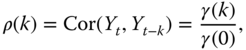
Figure 5.3 studies a time series of squares of logarithmic returns, computed from the daily S&P 500 data, which is described in Section 2.4.1. The squared logarithmic returns are often modeled as a stationary GARCH(![]() ) time series. However, we can also model the squared logarithmic returns with a signal plus noise model
) time series. However, we can also model the squared logarithmic returns with a signal plus noise model
where ![]() ,
, ![]() is a deterministic trend, and
is a deterministic trend, and ![]() is stationary white noise. We can estimate the trend
is stationary white noise. We can estimate the trend ![]() with a moving average
with a moving average ![]() . Moving averages are defined in Section 6.1.1. Panel (a) shows time series
. Moving averages are defined in Section 6.1.1. Panel (a) shows time series ![]() (black circles) and
(black circles) and ![]() (red line). Panel (b) shows
(red line). Panel (b) shows ![]() . Panel (b) suggests that subtracting the moving average could lead to stationarity. We use the one-sided exponential moving average in (6.3) with smoothing parameter
. Panel (b) suggests that subtracting the moving average could lead to stationarity. We use the one-sided exponential moving average in (6.3) with smoothing parameter ![]() .
.
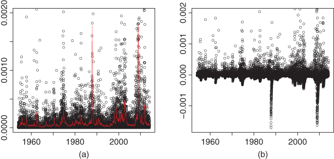
Figure 5.3 Removing a trend: Subtracting a moving average. (a) A times series of squared returns and a moving average of squared returns (red); (b) squared returns minus the moving average of squared returns.
5.1.1.1 Random Walk
Random walk is a discrete time stochastic process ![]() defined by
defined by
where ![]() is a random variable or a fixed value, and
is a random variable or a fixed value, and ![]() is distributed as IID(
is distributed as IID(![]() ). We have that
). We have that

If ![]() is a constant, then
is a constant, then ![]() and
and ![]() . Thus, random walk is not strictly stationary (and not covariance stationary). We obtain a Gaussian random walk if
. Thus, random walk is not strictly stationary (and not covariance stationary). We obtain a Gaussian random walk if ![]() is Gaussian white noise. If
is Gaussian white noise. If ![]() , then a Gaussian random walk satisfies
, then a Gaussian random walk satisfies ![]() .
.
Figure 5.4(a) shows the time series of S&P 500 prices over a period of 100 days. Panel (b) shows a simulated Gaussian random walk of length 100, when the initial value is 0. A random walk leads to a time series that has a stochastic trend. A stochastic trend is difficult to distinguish from a deterministic trend. A time series of stock prices resembles a random walk. Also a time series of a dividend price ratio in Figure 6.7(a) resembles a random walk.

Figure 5.4 Stochastic trend. (a) Prices of S&P 500 over 100 days; (b) simulated random walk of length 100, when the initial value is 0.
Geometric random walk is a discrete time stochastic process defined by

where ![]() are i.i.d and
are i.i.d and ![]() is independent of
is independent of ![]() .
.
5.1.2 Covariance Stationarity and Autocorrelation
We define autocovariance and autocorrelation first for scalar time series and then for vector time series.
5.1.2.1 Autocovariance and Autocorrelation for Scalar Time Series
We say that a time series ![]() is covariance stationary, if
is covariance stationary, if ![]() is a constant, not depending on
is a constant, not depending on ![]() , and
, and ![]() depends only on
depends only on ![]() but not on
but not on ![]() . A covariance stationary time series is called also second-order stationary.
. A covariance stationary time series is called also second-order stationary.
If ![]() for all
for all ![]() , then strict stationary implies covariance stationarity. There exists time series that are strictly stationary but for which covariance is not defined.2 Covariance stationarity does not imply strict stationarity. For a Gaussian time series, strict stationarity and covariance stationarity are equivalent. By a Gaussian time series, we mean a time series whose all finite dimensional marginal distributions have a Gaussian distribution.
, then strict stationary implies covariance stationarity. There exists time series that are strictly stationary but for which covariance is not defined.2 Covariance stationarity does not imply strict stationarity. For a Gaussian time series, strict stationarity and covariance stationarity are equivalent. By a Gaussian time series, we mean a time series whose all finite dimensional marginal distributions have a Gaussian distribution.
For a covariance stationary time series the autocovariance function is defined by
where ![]() . The covariance stationarity implies that
. The covariance stationarity implies that ![]() depends only on
depends only on ![]() and not on
and not on ![]() . The autocorrelation function is defined as
. The autocorrelation function is defined as
where ![]() .
.
The sample autocovariance with lag ![]() , based on the observations
, based on the observations ![]() , is defined as
, is defined as

where ![]() .3 The sample autocorrelation with lag
.3 The sample autocorrelation with lag ![]() is defined as
is defined as

Figure 5.5 shows sample autocorrelation functions for the daily S&P 500 index data, described in Section 2.4.1. Panel (a) shows the sample autocorrelation function ![]() for the return time series
for the return time series ![]() and panel (b) shows the sample autocorrelation function for the time series of the absolute returns
and panel (b) shows the sample autocorrelation function for the time series of the absolute returns ![]() . The lags are on the range
. The lags are on the range ![]() .
.

Figure 5.5 S&P 500 autocorrelation. (a) The sample autocorrelation function  of S&P 500 returns for
  ; (b) the sample autocorrelation function for absolute returns. The red lines indicate the 95% confidence band for the null hypothesis of i.i.d process.
If ![]() are i.i.d. with mean zero, then
are i.i.d. with mean zero, then
as ![]() ; see Brockwell and Davis (1991). Thus, if
; see Brockwell and Davis (1991). Thus, if ![]() are i.i.d. with mean zero, then about
are i.i.d. with mean zero, then about ![]() of the observed values
of the observed values ![]() should be inside the band
should be inside the band
where ![]() is the
is the ![]() -quantile for the standard normal distribution. Figure 5.5 has the red lines at the heights
-quantile for the standard normal distribution. Figure 5.5 has the red lines at the heights ![]() , where we have chosen
, where we have chosen ![]() , so that
, so that ![]() .
.
The Box–Ljung test can be used to test whether the autocorrelations are zero for a stationary time series ![]() . The null hypothesis is that
. The null hypothesis is that ![]() for
for ![]() , where
, where ![]() . Let us have observed time series
. Let us have observed time series ![]() . The test statistics is
. The test statistics is

where ![]() is defined in (5.3). The test rejects the null hypothesis of zero autocorrelations if
is defined in (5.3). The test rejects the null hypothesis of zero autocorrelations if
where ![]() is the
is the ![]() -quantile of the
-quantile of the ![]() -distribution with degrees of freedom
-distribution with degrees of freedom ![]() . We can compute the observed
. We can compute the observed ![]() -values
-values
for ![]() , where
, where ![]() is the distribution function of the
is the distribution function of the ![]() -distribution with degrees of freedom
-distribution with degrees of freedom ![]() . Small observed
. Small observed ![]() -values indicate that the observations are not compatible with the null hypothesis.
-values indicate that the observations are not compatible with the null hypothesis.
5.1.2.2 Autocovariance for Vector Time Series
Let ![]() be a vector time series with two components. Vector time series
be a vector time series with two components. Vector time series ![]() is covariance stationary when the components
is covariance stationary when the components ![]() and
and ![]() are covariance stationary and
are covariance stationary and
for all ![]() . Thus, vector time series
. Thus, vector time series ![]() is covariance stationary when
is covariance stationary when ![]() is a vector of constants, not depending on
is a vector of constants, not depending on ![]() , and the covariance
, and the covariance

depends only on ![]() but not on
but not on ![]() for
for ![]() .
.
For a covariance stationary time series the autocovariance function is defined by
For a scalar covariance stationary time series ![]() we have
we have
However, the autocovariance function of a vector time series satisfies4
5.2 Model Free Estimation
Univariate and multivariate descriptive statistics and graphical tools can be applied to get insight into a distribution of a time series. We can apply ![]() -variate descriptive statistics and graphical tools to the
-variate descriptive statistics and graphical tools to the ![]() -dimensional marginal distributions of a time series. This is discussed in Section 5.2.1.
-dimensional marginal distributions of a time series. This is discussed in Section 5.2.1.
Univariate and multivariate density estimators and regression estimators can be applied to time series data. We can apply ![]() -variate estimators to the
-variate estimators to the ![]() -dimensional marginal distributions of a time series. This is discussed in Section 5.2.2, by assuming that the time series is a Markov process of order
-dimensional marginal distributions of a time series. This is discussed in Section 5.2.2, by assuming that the time series is a Markov process of order ![]() .
.
Section 5.2.3 considers modeling time series with a combination of parametric and nonparametric methods. First a static parametric model is posed on the observations and then the time dynamics is introduced with time space or state space smoothing. The approach includes both local likelihood, covered in Section 5.2.3.1, and local least squares method, covered in Section 5.2.3.2. We apply local likelihood and local least squares to estimate time varying tail index in Section 5.2.3.3.
5.2.1 Descriptive Statistics for Time Series
Univariate statistics, as defined in Section 3.1, can be used to describe time series data ![]() . Using univariate statistics, like sample mean and sample variance, is reasonable if
. Using univariate statistics, like sample mean and sample variance, is reasonable if ![]() are identically distributed.
are identically distributed.
Multivariate statistics, as defined in Section 4.1, can be used to describe vector time series data ![]() . Again, the use of multivariate statistics like sample correlation is reasonable if
. Again, the use of multivariate statistics like sample correlation is reasonable if ![]() are identically distributed.
are identically distributed.
Multivariate statistics can be used also for univariate time series data ![]() if we create a vector time series from the initial univariate time series. We can create a two-dimensional vector time series by defining
if we create a vector time series from the initial univariate time series. We can create a two-dimensional vector time series by defining
for some ![]() . Now we can compute a sample correlation coefficient, for example, from data
. Now we can compute a sample correlation coefficient, for example, from data ![]() . This is reasonable if
. This is reasonable if ![]() are identically distributed. The requirement that
are identically distributed. The requirement that ![]() in (5.7) are identically distributed follows from strict stationarity of
in (5.7) are identically distributed follows from strict stationarity of ![]() .
.
5.2.2 Markov Models
We have defined strict stationarity in Section 5.1.1. A strictly stationary time series ![]() can be defined by giving all finite dimensional marginal distributions. That is, to define the distribution of a strictly stationary time series we need to define the distributions
can be defined by giving all finite dimensional marginal distributions. That is, to define the distribution of a strictly stationary time series we need to define the distributions
for all ![]() . If the time series is IID(0,
. If the time series is IID(0,![]() ), then we need only to define the distribution of
), then we need only to define the distribution of ![]() . We say that the time series is a Markov process, if
. We say that the time series is a Markov process, if
To define a Markov process we need to define the distribution of ![]() and
and ![]() . More generally, we say that the time series is a Markov process of order
. More generally, we say that the time series is a Markov process of order ![]() , if
, if
To define a Markov process of order ![]() we need to define the distributions of
we need to define the distributions of ![]() ,
, ![]() , …,
, …, ![]() .
.
To estimate nonparametrically the distribution of a Markov process of order ![]() , we can estimate the distributions of
, we can estimate the distributions of ![]() ,
, ![]() , …,
, …, ![]() nonparametrically.
nonparametrically.
5.2.3 Time Varying Parameter
Let ![]() be a time series. Let
be a time series. Let ![]() be a density function, where
be a density function, where ![]() is a parameter, and
is a parameter, and ![]() . We could ignore the time series properties and assume that
. We could ignore the time series properties and assume that ![]() are independent and identically distributed with density
are independent and identically distributed with density ![]() .
.
However, we can assume that parameter ![]() changes in time. Then the observations are not identically distributed, but
changes in time. Then the observations are not identically distributed, but ![]() has density
has density ![]() . In practice, we do not specify any dynamics for
. In practice, we do not specify any dynamics for ![]() , but construct estimates
, but construct estimates ![]() using nonparametric smoothing.
using nonparametric smoothing.
Note that even when we would assume independent and identically distributed observations, with time series data the parameter estimate is changing in time, because at time ![]() the estimate
the estimate ![]() is constructed using data
is constructed using data ![]() . This is called sequential estimation.
. This is called sequential estimation.
5.2.3.1 Local Likelihood
If ![]() are independent with density
are independent with density ![]() , then the density of
, then the density of ![]() is
is

The maximum likelihood estimator of ![]() is the value
is the value ![]() maximizing
maximizing

over ![]() . We can find a time varying estimator
. We can find a time varying estimator ![]() using either time space or state space localization. The local likelihood approach has been studied in Spokoiny (2010). The localization is discussed more in Sections 6.1.1 and 6.1.2.
using either time space or state space localization. The local likelihood approach has been studied in Spokoiny (2010). The localization is discussed more in Sections 6.1.1 and 6.1.2.
Time Space Localization
Let

where ![]() is the smoothing parameter and
is the smoothing parameter and ![]() is a kernel function. For example, we can take
is a kernel function. For example, we can take ![]() . Let
. Let ![]() be the value maximizing
be the value maximizing

over ![]() .
.
For example, let us consider the model
where ![]() are i.i.d. Denote
are i.i.d. Denote ![]() and
and ![]() , where
, where ![]() is the density of the standard normal distribution. Let
is the density of the standard normal distribution. Let ![]() . Now
. Now

Then ![]() , where
, where

State Space Localization
Let us observe the state variables ![]() in addition to observing time series
in addition to observing time series ![]() . Let
. Let

where ![]() is the smoothing parameter and
is the smoothing parameter and ![]() is a kernel function. We can take
is a kernel function. We can take ![]() the density of the standard normal distribution. Let
the density of the standard normal distribution. Let ![]() be the value maximizing (5.9) over
be the value maximizing (5.9) over ![]() .
.
For example, let us consider the model
where ![]() are i.i.d. The model can be written as
are i.i.d. The model can be written as
Denote ![]() and
and ![]() , where
, where ![]() is the density of the standard normal distribution. Then
is the density of the standard normal distribution. Then ![]() , as defined in (5.10).
, as defined in (5.10).
5.2.3.2 Local Least Squares
Let us consider a linear model with time changing parameters. Let us observe the explanatory variables ![]() in addition to observing time series
in addition to observing time series ![]() . Consider the model
. Consider the model
where ![]() ,
, ![]() are time dependent constants,
are time dependent constants, ![]() is the vector of explanatory variables, and
is the vector of explanatory variables, and ![]() is an error term.
is an error term.
We define the estimates of the time varying regression coefficients as the values ![]() and
and ![]() minimizing
minimizing

where ![]() is the time space localized weight defined in (5.8). When we observe in addition the state variables
is the time space localized weight defined in (5.8). When we observe in addition the state variables ![]() , then we can use the state space localized weight
, then we can use the state space localized weight ![]() , defined in (5.11).
, defined in (5.11).
5.2.3.3 Time Varying Estimators for the Excess Distribution
We discussed tail modeling in Section 3.4. The idea in tail modeling is to fit a parametric model only to the data in the left tail or to the data in the right tail. We can add time space or state space localization to the tail modeling. As before, ![]() is a time series.
is a time series.
Local Likelihood in Tail Estimation
Let family ![]() ,
, ![]() , model the excess distribution of a return distribution, where
, model the excess distribution of a return distribution, where ![]() . This means that if
. This means that if ![]() is the density of the return distribution then we assume for the left tail that
is the density of the return distribution then we assume for the left tail that
for some ![]() , where
, where ![]() , and
, and ![]() is the
is the ![]() th quantile of the return density:
th quantile of the return density: ![]() . For the right tail the corresponding assumption is
. For the right tail the corresponding assumption is
for some ![]() , where
, where ![]() , and
, and ![]() is the
is the ![]() th quantile of the return density:
th quantile of the return density: ![]() .
.
The local maximum likelihood estimator for the parameter of the left tail is obtained from (3.63) as

where ![]() is the empirical quantile computed from
is the empirical quantile computed from ![]() ,
, ![]() , and
, and
The time space localized weights ![]() are modified from (5.8) as
are modified from (5.8) as

where ![]() is the smoothing parameter and
is the smoothing parameter and ![]() is a kernel function. If there is available the state variables
is a kernel function. If there is available the state variables ![]() , then we can use the state space localized weights, modified from (5.11) as
, then we can use the state space localized weights, modified from (5.11) as

where ![]() is the smoothing parameter and
is the smoothing parameter and ![]() is a kernel function.
is a kernel function.
The local maximum likelihood estimator for the parameter of the right tail is obtained from (3.64) as

where ![]() is the empirical quantile,
is the empirical quantile, ![]() , and
, and
The weights are obtained from (5.13) and (5.14) by replacing ![]() with
with ![]() .
.
For example, let us assume that the excess distribution is the Pareto distribution, as defined in (3.74) as
where ![]() is the shape parameter. The maximum likelihood estimator has the closed form expression (3.75). The local maximum likelihood estimators are
is the shape parameter. The maximum likelihood estimator has the closed form expression (3.75). The local maximum likelihood estimators are
and

where ![]() , and
, and ![]() . For the left tail we assume that
. For the left tail we assume that ![]() , and for the right tail we assume that
, and for the right tail we assume that ![]() . These are the time varying Hill's estimators.
. These are the time varying Hill's estimators.
Figure 5.6 studies time varying Hill's estimates for the S&P 500 daily data, described in Section 2.4.1. Panel (a) shows the estimates for the left tail index and panel (b) shows the estimates for the right tail index. Sequentially calculated Hill's estimates are shown in black, time localized Hill's estimates with ![]() are shown in blue, and the case with
are shown in blue, and the case with ![]() is shown in yellow. The exponential kernel function is used. The estimation is started after there are 4 years of data. The tails are defined by the empirical quantile
is shown in yellow. The exponential kernel function is used. The estimation is started after there are 4 years of data. The tails are defined by the empirical quantile ![]() with
with ![]() and
and ![]() .
.

Figure 5.6 Time varying Hill's estimator. (a) Left tail index; (b) right tail index. The black curves show sequentially calculated Hill's estimates, the blue curves show the time localized estimates with  and the yellow curves have
  .
.
Time Varying Regression Estimator for Tail Index
Let ![]() be the observed time series at time
be the observed time series at time ![]() . The regression estimator for the parameter
. The regression estimator for the parameter ![]() of the Pareto distribution is given in (3.77). Let
of the Pareto distribution is given in (3.77). Let
The local regression estimator of the parameter of the left tail is

where ![]() is the empirical quantile and we assume
is the empirical quantile and we assume ![]() . The weights
. The weights ![]() are obtained from (5.13) and (5.14) by replacing index
are obtained from (5.13) and (5.14) by replacing index ![]() with the index
with the index ![]() , so that the weights correspond to the ordering
, so that the weights correspond to the ordering ![]() .
.
The local regression estimator of the parameter of the right tail is

where ![]() are the observations in reverse order,
are the observations in reverse order,
![]() is the empirical quantile,
is the empirical quantile, ![]() , and we assume
, and we assume ![]() .
.
Figure 5.7 studies time varying regression estimates for the tail index using the S&P 500 daily data, described in Section 2.4.1. Panel (a) shows the estimates for the left tail index and panel (b) shows the estimates for the right tail index. Sequentially calculated regression estimates are shown in black, time localized estimates with ![]() are shown in blue, and the case with
are shown in blue, and the case with ![]() is shown in yellow. The standard Gaussian kernel function is used. The estimation is started after there are 4 years of data. The tails are defined by the empirical quantile
is shown in yellow. The standard Gaussian kernel function is used. The estimation is started after there are 4 years of data. The tails are defined by the empirical quantile ![]() with
with ![]() and
and ![]() .
.

Figure 5.7 Time varying regression estimator. Time series of estimates of the tail index are shown. (a) Left tail index; (b) right tail index. The black curves show sequentially calculated regression estimates, the blue curves show the time localized estimates with  and the yellow curves have
  .
.
5.3 Univariate Time Series Models
We discuss first ARMA (autoregressive moving average) processes and after that we discuss conditional heteroskedasticity models. Conditional heteroskedasticity models include ARCH (autoregressive conditional heteroskedasticity) and GARCH (generalized autoregressive conditional heteroskedasticity) models. The ARMA, ARCH, and GARCH processes are discrete time stochastic processes. We discuss also continuous time stochastic processes, because geometric Brownian motion and related continuous time stochastic processes are widely used in option pricing.
Brockwell and Davis (1991) give a detailed presentation of linear time series analysis, Fan and Yao (2005) give a short introduction to ARMA models and a more detailed discussion of nonlinear models. Shiryaev (1999) presents results of time series analysis that are useful for finance.
5.3.1 Prediction and Conditional Expectation
Our presentation of discrete time series analysis is directed towards giving prediction formulas: these prediction formulas are used in Chapter 7 to provide benchmarks for the evaluation of the methods of volatility prediction. Chapter 6 studies nonparametric prediction.
Let ![]() be a time series with
be a time series with ![]() . We take the conditional expectation
. We take the conditional expectation
to be the best prediction of ![]() , given the observations
, given the observations ![]() , where
, where ![]() is the prediction step. Using the conditional expectation as the best predictor can be justified by the fact that the conditional expectation minimizes the mean squared error. In fact, the function
is the prediction step. Using the conditional expectation as the best predictor can be justified by the fact that the conditional expectation minimizes the mean squared error. In fact, the function ![]() minimizing
minimizing
is the conditional expectation: ![]() .5
.5
Besides predicting the value ![]() , we consider also predicting the squared value
, we consider also predicting the squared value ![]() .
.
In the following text, we give expressions for ![]() in the ARMA models and for
in the ARMA models and for ![]() in the ARCH and GARCH models. These expressions depend on the unknown parameters of the models. In order to apply the expressions we need to estimate the unknown parameters and insert the estimates into the expressions.
in the ARCH and GARCH models. These expressions depend on the unknown parameters of the models. In order to apply the expressions we need to estimate the unknown parameters and insert the estimates into the expressions.
The conditional expectation whose condition is the infinite past is a function ![]() of the infinite past. Since we have available only a finite number of observations, we have to truncate these functions to obtain a function
of the infinite past. Since we have available only a finite number of observations, we have to truncate these functions to obtain a function ![]() . It would be more useful to obtain formulas for
. It would be more useful to obtain formulas for
and
However, these formulas are more difficult to derive than the formulas where the condition of the conditional expectation is the infinite past.
5.3.2 ARMA Processes
ARMA processes are defined in terms of an innovation process. After defining innovation processes, we define MA (moving average) processes and AR (autoregressive) processes. ARMA processes are obtained by combining autoregressive and moving average processes.
5.3.2.1 Innovation Processes
Innovation processes are used to build more complex processes, like ARMA and GARCH processes. We define two innovation processes: a white noise process and an i.i.d. process.
We say that ![]() is a white noise process and write
is a white noise process and write ![]() if
if
- 1.
 ,
, - 2.
 ,
, - 3.
 for
for  ,
,
where ![]() is a constant. A white noise is a Gaussian white noise if
is a constant. A white noise is a Gaussian white noise if ![]() .
.
We say that ![]() is an i.i.d. process and write
is an i.i.d. process and write ![]() if
if
- 1.
 ,
, - 2.
 ,
, - 3.
 and
and  are independent for
  .
.
An i.i.d. process is also a white noise process. A Gaussian white noise is also an i.i.d. process.
5.3.2.2 Moving Average Processes
We define first a moving average process of a finite order, then we give prediction formulas, and finally define a moving average process of infinite order.
MA( ) Process
We use MA(![]() ) as a shorthand notation for a moving average process of order
) as a shorthand notation for a moving average process of order ![]() . A moving average process
. A moving average process ![]() of order
of order ![]() is a process satisfying
is a process satisfying
where ![]() ,
, ![]() is a white noise process, and
is a white noise process, and ![]() .
.
Figure 5.8 illustrates the definition of MA(![]() ) processes. In panel (a)
) processes. In panel (a) ![]() and in panel (b)
and in panel (b) ![]() . When
. When ![]() , then
, then ![]() and
and ![]() have one common white noise-term, but
have one common white noise-term, but ![]() and
and ![]() do not have common white noise-terms. When
do not have common white noise-terms. When ![]() , then
, then ![]() and
and ![]() have two common white noise-terms,
have two common white noise-terms, ![]() and
and ![]() have one common white noise-term, and
have one common white noise-term, and ![]() and
and ![]() do not have common white noise-terms.
do not have common white noise-terms.

Figure 5.8 The definition of a MA( ) process. (a) MA(
 ) process; (b) MA(
 ) process.
We have that
and

where ![]() . Thus, MA(
. Thus, MA(![]() ) process is such that a correlation exists between
) process is such that a correlation exists between ![]() and
and ![]() only if
only if ![]() . Equations (5.19) and (5.20) show that MA(
. Equations (5.19) and (5.20) show that MA(![]() ) process is covariance stationary.
) process is covariance stationary.
If we are given a covariance function ![]() , which is such that
, which is such that ![]() for
for ![]() , we can construct a MA(
, we can construct a MA(![]() ) process with this covariance function by solving
) process with this covariance function by solving ![]() and
and ![]() from the
from the ![]() equations
equations

Prediction of MA Processes
The conditional expectation ![]() is the best prediction of
is the best prediction of ![]() for
for ![]() , given the infinite past
, given the infinite past ![]() , in the sense of the mean squared prediction error, as we mentioned in Section 5.3.1. We denote
, in the sense of the mean squared prediction error, as we mentioned in Section 5.3.1. We denote ![]() . The best linear prediction in the sense of the mean squared error is given in (6.19). We can use that formula when the covariance function of the MA(
. The best linear prediction in the sense of the mean squared error is given in (6.19). We can use that formula when the covariance function of the MA(![]() ) process is first estimated.
) process is first estimated.
A recursive prediction formula for the MA(![]() ) process can be derived as follows. We have that
) process can be derived as follows. We have that

because ![]() for
for ![]() . The noise terms
. The noise terms ![]() are not observed, but we can write
are not observed, but we can write

This leads to a formula for ![]() in terms of the infinite past
in terms of the infinite past ![]() . For example, for the MA(1) process
. For example, for the MA(1) process ![]() we have
we have

The prediction formula for prediction step ![]() is a version of exponential moving average, which is defined in (6.7).
is a version of exponential moving average, which is defined in (6.7).
We can obtain a recursive prediction for practical use in the following way. Define ![]() , when
, when ![]() and
and
when ![]() . Finally we define the
. Finally we define the ![]() -step prediction as
-step prediction as
For example, for the MA(1) process ![]() we get the truncated formulas
we get the truncated formulas

In the implementation the parameters ![]() have to be replaced by their estimates.
have to be replaced by their estimates.
MA( ) Process
A moving average process of infinite order is defined as

The series converges in mean square if6

We have that

and
Equations (5.22) and (5.23) imply that MA(![]() ) process is covariance stationary. MA(
) process is covariance stationary. MA(![]() ) process can be used to study the properties of AR processes. For example, if we can write an AR process as a MA(
) process can be used to study the properties of AR processes. For example, if we can write an AR process as a MA(![]() ) process, this shows that the AR process is covariance stationary.
) process, this shows that the AR process is covariance stationary.
5.3.2.3 Autoregressive Processes
An autoregressive process ![]() of order
of order ![]() is a process satisfying
is a process satisfying
where ![]() ,
, ![]() is a white noise process, and
is a white noise process, and ![]() . We assume that
. We assume that ![]() is uncorrelated with
is uncorrelated with ![]() . We use AR(
. We use AR(![]() ) as a shorthand notation for an autoregressive process of order
) as a shorthand notation for an autoregressive process of order ![]() .
.
The autocovariance function of an AR(![]() ) process can be computed recursively. Multiply (5.24) by
) process can be computed recursively. Multiply (5.24) by ![]() from both sides and take expectations to get
from both sides and take expectations to get
where ![]() . The first values
. The first values ![]() can be solved from the
can be solved from the ![]() equations. After that, the values
equations. After that, the values ![]() for
for ![]() can be computed recursively from (5.25).
can be computed recursively from (5.25).
Prediction of AR Processes
Let us consider the prediction of ![]() for
for ![]() when the process is an AR(
when the process is an AR(![]() ) process. The best prediction of
) process. The best prediction of ![]() , given the observations
, given the observations ![]() , is denoted by
, is denoted by
where we denote ![]() . We start with the one-step prediction. The best prediction of
. We start with the one-step prediction. The best prediction of ![]() , given the observations
, given the observations ![]() , is
, is
because ![]() . For the two-step prediction the best predictor is
. For the two-step prediction the best predictor is

The general prediction formula is
The best prediction is calculated recursively, using the value of ![]() in (5.26), and the fact that
in (5.26), and the fact that ![]() for
for ![]() .
.
For example, for the MA(1) process ![]() we have
we have
5.3.2.4 ARMA Processes
We define an autoregressive moving average process ![]() , of order
, of order ![]() ,
, ![]() , as a process satisfying
, as a process satisfying
where ![]() and
and ![]() is a MA(
is a MA(![]() ) process. We use ARMA(
) process. We use ARMA(![]() ) as a shorthand notation for an autoregressive moving average process of order (
) as a shorthand notation for an autoregressive moving average process of order (![]() ).
).
Stationarity, Causality, and Invertability of ARMA Processes
Let ![]() be an ARMA(
be an ARMA(![]() ) process with
) process with
Denote

where ![]() , and
, and ![]() is the set of complex numbers. If
is the set of complex numbers. If ![]() for all
for all ![]() such that
such that ![]() , then there exists the unique stationary solution
, then there exists the unique stationary solution

where the coefficients ![]() are obtained from the equation
are obtained from the equation

where ![]() for some
for some ![]() ; see Brockwell and Davis (1991, Theorem 3.1.3).
; see Brockwell and Davis (1991, Theorem 3.1.3).
The condition for the covariance stationarity does not guarantee that the ARMA(![]() ) process would be suitable for modeling. Let us consider the AR(1) model
) process would be suitable for modeling. Let us consider the AR(1) model
where ![]() . The AR(1) model is covariance stationary if and only if
. The AR(1) model is covariance stationary if and only if ![]() . This can be seen in the following way. Let us consider first the case
. This can be seen in the following way. Let us consider first the case ![]() . We can write recursively
. We can write recursively

where ![]() . Since
. Since ![]() , we get the MA(
, we get the MA(![]() ) representation7
) representation7

which implies that ![]() is covariance stationary. Let us then consider the case
is covariance stationary. Let us then consider the case ![]() . Since
. Since ![]() , we can write recursively
, we can write recursively

where ![]() . Since
. Since ![]() , we get the MA(
, we get the MA(![]() ) representation8
) representation8

which implies that ![]() is covariance stationary. The latter case
is covariance stationary. The latter case ![]() is not suitable for modeling because
is not suitable for modeling because ![]() is a function of future innovations
is a function of future innovations ![]() with
with ![]() .
.
We define causality of the process to exclude examples like the AR(1) model with ![]() . An ARMA(
. An ARMA(![]() ) process is called causal if there exists constants
) process is called causal if there exists constants ![]() such that
such that ![]() and
and

Let the polynomials ![]() and
and ![]() have no common zeroes. Then
have no common zeroes. Then ![]() is causal if and only if
is causal if and only if ![]() for all
for all ![]() such that
such that ![]() .9 This has been proved in Brockwell and Davis (1991, Theorem 3.1.1). The coefficients
.9 This has been proved in Brockwell and Davis (1991, Theorem 3.1.1). The coefficients ![]() are determined by
are determined by

Thus, under the conditions that ![]() and
and ![]() have no common zeroes and
have no common zeroes and ![]() for all
for all ![]() such that
such that ![]() , we have expressed an ARMA(
, we have expressed an ARMA(![]() ) process as an infinite order moving average process. Thus, an ARMA(
) process as an infinite order moving average process. Thus, an ARMA(![]() ) process is covariance stationary under these conditions.
) process is covariance stationary under these conditions.
An ARMA(![]() ) process is called invertible if there exists constants
) process is called invertible if there exists constants ![]() such that
such that ![]() and
and

Let the polynomials ![]() and
and ![]() have no common zeroes. Then
have no common zeroes. Then ![]() is invertible if and only if
is invertible if and only if ![]() for all
for all ![]() such that
such that ![]() . This has been proved in Brockwell and Davis (1991, Theorem 3.1.2). The coefficients
. This has been proved in Brockwell and Davis (1991, Theorem 3.1.2). The coefficients ![]() are determined by
are determined by
Prediction of ARMA Processes
The prediction formulas for ARMA processes given the infinite past can be found in Hamilton (1994, p. 77). For the ARMA (1,1) process ![]() we have
we have

where ![]() ; see Shiryaev (1999, p. 151). Note that the prediction formula (5.21) of the MA(1) process and the prediction formula (5.27) of the AR(1) process follow from (5.28).
; see Shiryaev (1999, p. 151). Note that the prediction formula (5.21) of the MA(1) process and the prediction formula (5.27) of the AR(1) process follow from (5.28).
5.3.3 Conditional Heteroskedasticity Models
Time series ![]() satisfies the conditional heteroskedasticity assumption if
satisfies the conditional heteroskedasticity assumption if
where ![]() is an IID(
is an IID(![]() ) process and
) process and ![]() is the volatility process. The volatility process is a predictable random process, that is,
is the volatility process. The volatility process is a predictable random process, that is, ![]() is measurable with respect to the sigma-field
is measurable with respect to the sigma-field ![]() generated by the variables
generated by the variables ![]() . We also assume that
. We also assume that ![]() is independent of
is independent of ![]() . Then,
. Then,
Thus, ![]() is the best prediction of
is the best prediction of ![]() in the mean squared error sense. Also, for
in the mean squared error sense. Also, for ![]() ,
,

Thus, the best prediction of ![]() gives the best prediction of
gives the best prediction of ![]() , in the mean squared error sense.
, in the mean squared error sense.
ARCH and GARCH processes are examples of conditional heteroskedasticity models.
5.3.3.1 ARCH Processes
Process ![]() is an ARCH(
is an ARCH(![]() ) process (autoregressive conditional heteroskedasticity process of order
) process (autoregressive conditional heteroskedasticity process of order ![]() ), if
), if ![]() where
where ![]() is an IID(
is an IID(![]() ) process and
) process and

where ![]() and
and ![]() . As a special case, the ARCH
. As a special case, the ARCH![]() process is defined as
process is defined as
The ARCH model was introduced in Engle (1982) for modeling UK inflation rates. The ARCH(![]() ) process is strictly stationary if
) process is strictly stationary if ![]() ; see Fan and Yao (2005, Theorem 4.3) and Giraitis et al. (2000).
; see Fan and Yao (2005, Theorem 4.3) and Giraitis et al. (2000).
Let us consider the prediction of ![]() for
for ![]() when the process is an ARCH(
when the process is an ARCH(![]() ) process. The best prediction of
) process. The best prediction of ![]() , given the observations
, given the observations ![]() , is denoted by
, is denoted by
We start with the one-step prediction. The best prediction of ![]() , given the observations
, given the observations ![]() , using the inference in (5.30), is
, using the inference in (5.30), is

because ![]() . For the two-step prediction we use (5.30) to obtain the best predictor
. For the two-step prediction we use (5.30) to obtain the best predictor

The general prediction formula is

where we denote ![]() . The best prediction is calculated recursively, using the value of
. The best prediction is calculated recursively, using the value of ![]() in (5.33), and the fact that
in (5.33), and the fact that ![]() for
for ![]() .
.
The best ![]() -step prediction in the ARCH(1) model is
-step prediction in the ARCH(1) model is

where we assumed condition ![]() , which guarantees stationarity, and we denote
, which guarantees stationarity, and we denote ![]() .10
.10
5.3.3.2 GARCH Processes
Process ![]() is a GARCH(
is a GARCH(![]() ) process (generalized autoregressive conditional heteroskedasticity process of order
) process (generalized autoregressive conditional heteroskedasticity process of order ![]() and
and ![]() ), if
), if
where ![]() is an IID(
is an IID(![]() ) process and
) process and

where ![]() ,
, ![]() , and
, and ![]() . As a special case we get the GARCH
. As a special case we get the GARCH![]() model, where
model, where
The GARCH model was introduced in Bollerslev (1986). The GARCH(![]() ) process is strictly stationary if
) process is strictly stationary if

see Fan and Yao (2005, Theorem 4.4) and Bougerol and Picard (1992).
The best one-step prediction of the squared value is obtained from (5.30) as
In the GARCH(![]() ) model the best
) model the best ![]() -step prediction of the squared value, in the mean squared error sense, is
-step prediction of the squared value, in the mean squared error sense, is
where we assumed condition ![]() , which guarantees strict stationarity, and we denote the unconditional variance by
, which guarantees strict stationarity, and we denote the unconditional variance by
Let us show (5.40) for ![]() . Let us denote
. Let us denote ![]() . We have
. We have
and ![]() . Thus,
. Thus,
Thus, using (5.31),

We have shown (5.40), since ![]() , by (5.31). We can also write the best prediction of
, by (5.31). We can also write the best prediction of ![]() in the GARCH(
in the GARCH(![]() ) model as
) model as

where ![]() .
.
The prediction formulas (5.40) and (5.42) are written in terms of ![]() . We have the following formula for
. We have the following formula for ![]() in a strictly stationary GARCH(
in a strictly stationary GARCH(![]() ) model:
) model:
where we assume ![]() to ensure strict stationarity. More generally, for the GARCH(
to ensure strict stationarity. More generally, for the GARCH(![]() ) model we have
) model we have

where ![]() are obtained from the equation
are obtained from the equation

for ![]() ; see Fan and Yao (2005, Theorem 4.4).
; see Fan and Yao (2005, Theorem 4.4).
5.3.3.3 ARCH( ) Model
GARCH(![]() ) can be considered a special case of the ARCH(
) can be considered a special case of the ARCH(![]() ) model, since (5.43) can be written as
) model, since (5.43) can be written as

where ![]() and
and ![]() . We can obtain a more general ARCH (
. We can obtain a more general ARCH (![]() ) model by defining
) model by defining

where ![]() ,
, ![]() , and
, and ![]() is called a news impact curve. More generally, following Linton (2009), the news impact curve can be defined as the relationship between
is called a news impact curve. More generally, following Linton (2009), the news impact curve can be defined as the relationship between ![]() and
and ![]() holding past values
holding past values ![]() constant at some level
constant at some level ![]() . In the GARCH(
. In the GARCH(![]() ) model the news impact curve is
) model the news impact curve is
The ARCH(![]() ) model in (5.45) has been studied in Linton and Mammen (2005), where it was noted that the estimated news impact curve is asymmetric for S&P 500 return data. The asymmetric news impact curve can be addressed by asymmetric GARCH processes.
) model in (5.45) has been studied in Linton and Mammen (2005), where it was noted that the estimated news impact curve is asymmetric for S&P 500 return data. The asymmetric news impact curve can be addressed by asymmetric GARCH processes.
5.3.3.4 Asymmetric GARCH Processes
Time series of asset returns show a leverage effect. Markets become more active after a price drop: large negative returns are followed by a larger increase in volatility than in the case of large positive returns. In fact, past price changes and future volatilities are negatively correlated. This implies a negative skew to the distribution of the price changes.
The leverage effect is taken into account in the model

where ![]() is the skewness parameter. The model was applied in Heston and Nandi (2000) to price options.11
When
is the skewness parameter. The model was applied in Heston and Nandi (2000) to price options.11
When ![]() , then under (5.46)
, then under (5.46)
When ![]() , then negative values of
, then negative values of ![]() lead to larger increase in volatility than positive values of the same size of
lead to larger increase in volatility than positive values of the same size of ![]() . Now the unconditional variance is
. Now the unconditional variance is
5.3.3.5 The Moment Generating function
We need the moment generating function in order to compute the option prices when the stock follows an asymmetric GARCH(![]() ) process. We follow Heston and Nandi (2000). Let
) process. We follow Heston and Nandi (2000). Let
where ![]() ,
, ![]() ,
, ![]() are i.i.d.
are i.i.d. ![]() , and
, and
For example, when the logarithmic returns follow the asymmetric GARCH(![]() ) process, then
) process, then
so that ![]() . We want to find the moment generating function
. We want to find the moment generating function
where ![]() and
and ![]() is the conditional expectation at time
is the conditional expectation at time ![]() .
.
We have that
Also,
because the moment generating function of ![]() is
is ![]() , and
, and ![]() .
.
For ![]() we have
we have
where ![]() and
and ![]() are defined by the recursive formulas
are defined by the recursive formulas

The cases ![]() and
and ![]() were proved in (5.51) and (5.52). Let
were proved in (5.51) and (5.52). Let ![]() . Let us make the induction assumption that the formulas hold at time
. Let us make the induction assumption that the formulas hold at time ![]() . Now,
. Now,

Insert values

to get

When ![]() , then
, then

Equating terms in (5.54) and (5.55) gives the result.12
Figure 5.9 shows moment generating functions ![]() . In panel (a) the current stock price is
. In panel (a) the current stock price is ![]() , and in panel (b)
, and in panel (b) ![]() . The one period moment generating function (
. The one period moment generating function (![]() ) is with black, two period (
) is with black, two period (![]() ) is with red, and three period (
) is with red, and three period (![]() ) is with blue. The parameters
) is with blue. The parameters ![]() ,
, ![]() ,
, ![]() , and
, and ![]() are estimated from the daily S&P 500 daily data of Section 2.4.1, using model (5.46).
are estimated from the daily S&P 500 daily data of Section 2.4.1, using model (5.46).

Figure 5.9 Moment generating functions under GARCH. We show functions  , where (a)
  and (b)
  . The case
  is with black,
  is with red, and
  is with blue.
Note that under the usual GARCH(![]() ) model
) model
functions ![]() and
and ![]() are defined by the recursive formulas
are defined by the recursive formulas

This means that ![]() and
and ![]() depend on the unobserved sequence
depend on the unobserved sequence ![]() , unlike in the case of model (5.50).
, unlike in the case of model (5.50).
5.3.3.6 Parameter Estimation
We discuss first estimation of the ARCH processes, and then extend the discussion to the GARCH processes.
Parameter Estimation for ARCH Processes
Estimation of the parameters of ARCH(![]() ) model can be done using the method of maximum likelihood, if we make an assumption about the distribution of innovation
) model can be done using the method of maximum likelihood, if we make an assumption about the distribution of innovation ![]() . When we have observed
. When we have observed ![]() , then the likelihood function is
, then the likelihood function is
Let us ignore the term ![]() and define the conditional likelihood
and define the conditional likelihood

Let us denote the density of ![]() by
by ![]() . Then the conditional density of
. Then the conditional density of ![]() , given
, given ![]() , is
, is

where
The parameters are estimated by maximizing the conditional likelihood, and we get
where the logarithm of the conditional likelihood is

If we assume that ![]() has the standard normal distribution
has the standard normal distribution ![]() then
then ![]() and
and

Parameter Estimation for GARCH Processes
In the GARCH(![]() ) model we can use, similarly to (5.57),
) model we can use, similarly to (5.57),

where ![]() . Unlike in the ARCH
. Unlike in the ARCH![]() model,
model, ![]() is a sum of infinitely many terms, and we need to truncate the infinite sum in order to be able to calculate the conditional likelihood. The value
is a sum of infinitely many terms, and we need to truncate the infinite sum in order to be able to calculate the conditional likelihood. The value ![]() can be chosen as the sample variance using
can be chosen as the sample variance using ![]() , and
, and ![]() for
for ![]() can be computed using the recursive formula. Then
can be computed using the recursive formula. Then ![]() is a function of
is a function of ![]() and of the parameters.
and of the parameters.
5.3.3.7 Fitting the GARCH( ) Model
We fit the GARCH(![]() ) model for S&P 500 index and for individual stocks of S&P 500.
) model for S&P 500 index and for individual stocks of S&P 500.
S&P 500 Daily Data
Figure 5.10 shows tail plots of the residuals ![]() , where
, where ![]() is the estimated volatility in the GARCH(
is the estimated volatility in the GARCH(![]() ) model. Panel (a) shows the left tail plot and panel (b) the right tail plot. The black points show the residuals, the red curves show the standard normal distribution function, and the blue curves show the Student distributions with degrees of freedom 3, 6, and 12. Figure 3.2 shows the corresponding plots for the S&P 500 returns. We see that the standard normal distribution fits well the central area of the distribution of the residuals, but the tails may be better fitted with a Student distribution.
) model. Panel (a) shows the left tail plot and panel (b) the right tail plot. The black points show the residuals, the red curves show the standard normal distribution function, and the blue curves show the Student distributions with degrees of freedom 3, 6, and 12. Figure 3.2 shows the corresponding plots for the S&P 500 returns. We see that the standard normal distribution fits well the central area of the distribution of the residuals, but the tails may be better fitted with a Student distribution.

Figure 5.10 GARCH(1,1) residuals: Tail plots. (a) Left tail plot; (b) right tail plot. The red curves show the standard normal distribution function, and the blue curves show the Student distributions with degrees of freedom  ,
,  , and
, and  .
.
S&P 500 Components Data
We compute GARCH estimates for daily S&P 500 components data, described in Section 2.4.5. Estimates are computed both for the GARCH(![]() ) model and for the Heston–Nandi modification of the GARCH(
) model and for the Heston–Nandi modification of the GARCH(![]() ) model, defined in (5.46).13 Both models have parameters
) model, defined in (5.46).13 Both models have parameters ![]() ,
, ![]() , and
, and ![]() . The Heston–Nandi model has the additional skewness parameter
. The Heston–Nandi model has the additional skewness parameter ![]() .
.
Figure 5.11(a) shows a scatter plot of ![]() , where
, where ![]() are estimates of
are estimates of ![]() in the GARCH(
in the GARCH(![]() ) model and
) model and ![]() are estimates of
are estimates of ![]() in the Heston–Nandi model. The red points show the estimates for daily S&P 500 data, described in Section 2.4.1. Panel (b) shows a scatter plot of
in the Heston–Nandi model. The red points show the estimates for daily S&P 500 data, described in Section 2.4.1. Panel (b) shows a scatter plot of ![]() . We see that the estimates of
. We see that the estimates of ![]() are of the order
are of the order ![]() .
.
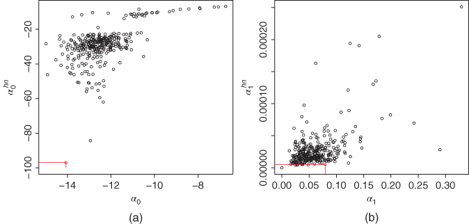
Figure 5.11 GARCH(1,1) estimates versus Heston–Nandi estimates:  and
and  . (a) A scatter plot of
  ; (b) a scatter plot of
  , where
  and
and  are estimates in the GARCH(
 ) model, and
  and
and  are estimates in the Heston–Nandi model.
Figure 5.12(a) shows a scatter plot of ![]() , where
, where ![]() are estimates of
are estimates of ![]() in the GARCH(
in the GARCH(![]() ) model, and
) model, and ![]() are estimates of
are estimates of ![]() in the Heston–Nandi model. We leave out outliers with small estimates for
in the Heston–Nandi model. We leave out outliers with small estimates for ![]() . Panel (b) shows a histogram of estimates
. Panel (b) shows a histogram of estimates ![]() of
of ![]() in the Heston–Nandi model. The red points and the lines show the estimates for daily S&P 500 data, described in Section 2.4.1. We see that estimates of
in the Heston–Nandi model. The red points and the lines show the estimates for daily S&P 500 data, described in Section 2.4.1. We see that estimates of ![]() are close to 1, and they are more linearly related in the two models than the estimates of
are close to 1, and they are more linearly related in the two models than the estimates of ![]() and
and ![]() . Also, we see that the estimates of the skewness parameter
. Also, we see that the estimates of the skewness parameter ![]() are positive for almost all S&P 500 components, with the median value about 2.5. This indicates that high negative returns increase volatility more than the positive returns.
are positive for almost all S&P 500 components, with the median value about 2.5. This indicates that high negative returns increase volatility more than the positive returns.
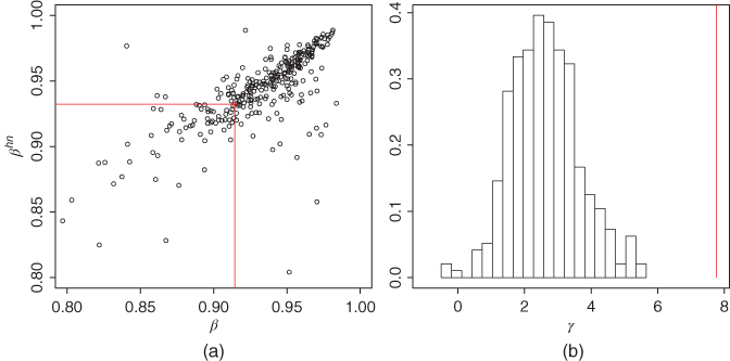
Figure 5.12 GARCH(1,1) estimates versus Heston–Nandi estimates:  and
and  . (a) A scatter plot of
  , where
  are estimates in the GARCH(
 ) model, and
  are estimates in the Heston–Nandi model. Panel (b) shows a histogram of estimates
  of
of  in the Heston–Nandi model.
5.3.4 Continuous Time Processes
The geometric Brownian motion is used to model stock prices in the Black–Scholes model. We do not go into details about continuous time models, but we think that it is useful to review some basic facts about continuous time models. In particular, the geometric Brownian motion appears as the limit of a discrete time binomial model.
5.3.4.1 The Brownian Motion
Stochastic process ![]() ,
, ![]() , is called the standard Brownian motion, or the standard Wiener process, if it has the following properties:
, is called the standard Brownian motion, or the standard Wiener process, if it has the following properties:
- 1.
 with probability one,
 - 2.
 ,
, - 3.
 is independent of
  for
for  .
.
The Brownian motion leads to the process
where ![]() is drift and
is drift and ![]() is volatility. We can use the notation of stochastic differential equations:
is volatility. We can use the notation of stochastic differential equations:
5.3.4.2 Diffusion Processes and Itô's Lemma
The diffusion Markov process is defined as

where ![]() ,
, ![]() is a random variable, and
is a random variable, and

with probability one; see Shiryaev (1999, p. 237). A definition of the stochastic integrals with respect to the Brownian motion can be found in Shiryaev (1999, p. 252).14 The definition of the process can be written with the shorthand notation of the stochastic differential equations:
For example, a mean reverting model is defined as
Let ![]() be a diffusion process as in (5.60), and let
be a diffusion process as in (5.60), and let ![]() , where
, where ![]() is continuously differentiable with respect to the first argument and two times continuously differentiable with respect to the second argument. Furthermore, we assume that
is continuously differentiable with respect to the first argument and two times continuously differentiable with respect to the second argument. Furthermore, we assume that ![]() . Then
. Then ![]() is a diffusion Markov process with
is a diffusion Markov process with
where

and ![]() ,
, ![]() , and
, and ![]() are related by
are related by ![]() . The expression for
. The expression for ![]() follows from Itô's lemma; see Shiryaev (1999, p. 263).15
follows from Itô's lemma; see Shiryaev (1999, p. 263).15
5.3.4.3 The Geometric Brownian Motion
The geometric Brownian motion is the stochastic process
where ![]() is the standard Brownian motion,
is the standard Brownian motion, ![]() , and
, and ![]() . The stochastic differential equation of the geometric Brownian motion is
. The stochastic differential equation of the geometric Brownian motion is
The fact that the solution of the stochastic differential equation in (5.63) is given in (5.62) follows from Itô's formula. Indeed, we consider diffusion process ![]() ,
, ![]() ,
, ![]() , and
, and ![]() . Then Itô's formula implies that
. Then Itô's formula implies that ![]() is a diffusion process with
is a diffusion process with ![]() and
and ![]() .
.
5.3.4.4 Girsanov's Theorem
Let ![]() be a filtered probability space and let
be a filtered probability space and let ![]() be a Brownian motion. Let
be a Brownian motion. Let ![]() be a stochastic process with
be a stochastic process with ![]() , for
, for ![]() . We construct a process
. We construct a process ![]() by setting
by setting

If ![]() , then
, then ![]() . We can define a probability measure
. We can define a probability measure ![]() on
on ![]() by
by
where ![]() . Let
. Let ![]() be the restriction of
be the restriction of ![]() to
to ![]() . Measure
. Measure ![]() is equivalent to
is equivalent to ![]() . Girsanov's theorem states that
. Girsanov's theorem states that

defines a Brownian motion ![]() ; see Shiryaev (1999, p. 269). A proof can be found in Shiryaev (1999, Chapter VII, Section 3b).
; see Shiryaev (1999, p. 269). A proof can be found in Shiryaev (1999, Chapter VII, Section 3b).
5.4 Multivariate Time Series Models
The multivariate GARCH model is defined for vector time series ![]() that has
that has ![]() components. It is assumed that
components. It is assumed that ![]() is strictly stationary and
is strictly stationary and
where ![]() is the square root of a positive definite covariance matrix
is the square root of a positive definite covariance matrix ![]() ,
, ![]() is measurable with respect to the sigma-algebra generated by
is measurable with respect to the sigma-algebra generated by ![]() , and
, and ![]() is a
is a ![]() -dimensional i.i.d. process with
-dimensional i.i.d. process with ![]() and
and ![]() , where
, where ![]() is the
is the ![]() identity matrix.
identity matrix.
The square root of ![]() can be defined by writing the eigenvalue decomposition
can be defined by writing the eigenvalue decomposition ![]() , where
, where ![]() is the diagonal matrix of the eigenvalues of
is the diagonal matrix of the eigenvalues of ![]() and
and ![]() is the orthogonal matrix whose columns are the eigenvectors of
is the orthogonal matrix whose columns are the eigenvectors of ![]() . Then we define
. Then we define ![]() , where
, where ![]() is the diagonal matrix obtained from
is the diagonal matrix obtained from ![]() by taking square root of each element. We can define
by taking square root of each element. We can define ![]() also as a Cholesky factor of
also as a Cholesky factor of ![]() .
.
Multivariate GARCH (MGARCH) processes are reviewed in McNeil et al. (2005, Section 4.6), Bauwens et al. (2006), and Silvennoinen and Teräsvirta (2009). Below we write the models only for the case ![]() , so that
, so that ![]() . The multivariate GARCH models are denoted with MGARCH(
. The multivariate GARCH models are denoted with MGARCH(![]() ). We restrict ourselves to the first-order models with
). We restrict ourselves to the first-order models with ![]() . The multivariate GARCH models are based on (5.65) but differ in the definition of the recursive formula for
. The multivariate GARCH models are based on (5.65) but differ in the definition of the recursive formula for ![]() .
.
5.4.1 MGARCH Models
First we define the VEC model and two restrictions of it: the diagonal VEC model and the Baba–Engle–Kraft–Kroner (BEKK) model. Then we define the constant correlation model and the dynamic conditional correlation model.
Let us denote ![]() ,
, ![]() , and
, and ![]() . The VEC model and the diagonal VEC model were introduced in Bollerslev et al. (1988). The VEC model assumes that
. The VEC model and the diagonal VEC model were introduced in Bollerslev et al. (1988). The VEC model assumes that

This model has 21 parameters ![]() . Since the model has a large number of parameters, it is useful to consider models with less parameters. The diagonal VEC model has only nine parameters and assumes that
. Since the model has a large number of parameters, it is useful to consider models with less parameters. The diagonal VEC model has only nine parameters and assumes that
Thus, in the diagonal VEC model the components of ![]() follow univariate GARCH models. The BEKK model was introduced in Engle and Kroner (1995). The model has 11 parameters and it can be written more easily with the matrix notation as
follow univariate GARCH models. The BEKK model was introduced in Engle and Kroner (1995). The model has 11 parameters and it can be written more easily with the matrix notation as
where ![]() is a symmetric
is a symmetric ![]() matrix and
matrix and ![]() and
and ![]() are
are ![]() matrices. The BEKK model is obtained from the VEC model by restricting the parameters. We can express the parameters
matrices. The BEKK model is obtained from the VEC model by restricting the parameters. We can express the parameters ![]() of the VEC model in terms of the parameters of the BEKK model as follows:
of the VEC model in terms of the parameters of the BEKK model as follows:

where we denote the elements of ![]() by
by ![]() and the elements of
and the elements of ![]() by
by ![]() .
.
The recursive formula for ![]() can be written by using the correlation matrix
can be written by using the correlation matrix ![]() . Let
. Let ![]() be the diagonal matrix of the standard deviations of
be the diagonal matrix of the standard deviations of ![]() . The correlation matrix
. The correlation matrix ![]() , corresponding to
, corresponding to ![]() , is such that
, is such that ![]() .
.
The constant correlation MGARCH model, introduced in Bollerslev (1990), is such that the components of ![]() follow univariate GARCH models, and the correlation matrix is constant. That is,
follow univariate GARCH models, and the correlation matrix is constant. That is, ![]() and
and ![]() , where
, where ![]() is the constant correlation matrix. The constant correlation GARCH model assumes the univariate GARCH models for the components, as in (5.66) and (5.67), and
is the constant correlation matrix. The constant correlation GARCH model assumes the univariate GARCH models for the components, as in (5.66) and (5.67), and
The dynamic conditional correlation MGARCH model, introduced in Engle (2002), is such that the components of ![]() follow univariate GARCH models and
follow univariate GARCH models and
where ![]() Engle (2002) suggests to estimate
Engle (2002) suggests to estimate
where ![]() is the sample covariance with
is the sample covariance with ![]() and
and ![]() . We do not typically have
. We do not typically have ![]() , and thus the conditional correlation is estimated from
, and thus the conditional correlation is estimated from

where ![]() and
and ![]() .
.
5.4.2 Covariance in MGARCH Models
The recursive equation (5.68) in the stationary diagonal VEC model implies that

This follows similarly as in the case of GARCH![]() model (see (5.43) and (5.44)). The recursive equation (5.69) in the stationary dynamic conditional correlation GARCH model implies similarly that
model (see (5.43) and (5.44)). The recursive equation (5.69) in the stationary dynamic conditional correlation GARCH model implies similarly that

where ![]() .
.
Given the observations ![]() , we estimate the parameters, similarly to GARCH(
, we estimate the parameters, similarly to GARCH(![]() ) estimation in (5.58), by maximizing the conditional modified likelihood,
) estimation in (5.58), by maximizing the conditional modified likelihood,

where ![]() ,
, ![]() is the density of the standard normal bivariate distribution
is the density of the standard normal bivariate distribution ![]() , and
, and ![]() is the truncated covariance, with elements
is the truncated covariance, with elements ![]() ,
, ![]() ,
, ![]() , where
, where

and ![]() ,
, ![]() are defined similarly.
are defined similarly.
Given the data ![]() , the MGARCH
, the MGARCH![]() estimator for the conditional covariance is
estimator for the conditional covariance is

where the parameter estimators ![]() ,
, ![]() , and
, and ![]() are are calculated with the maximum likelihood method.
are are calculated with the maximum likelihood method.
5.5 Time Series Stylized Facts
Time series models of financial time series should be such that they are able to capture stylized facts. We describe the stylized facts mainly using the daily S&P 500 index data, described in Section 2.4.1. Stylized facts of financial time series are studied by Cont (2001) and Bouchaud (2002).
- 1. Returns are uncorrelated.
Figure 5.5(a) shows the sample autocorrelation function for the S&P 500 returns. Sample autocorrelations are small, although they are not completely inside the 95% confidence band.
When the time scale is shorter than tens of minutes, there can be considerable correlation; see Cont (2001) and Bouchaud (2002).
- 2. Absolute returns are correlated.
Figure 5.5(b) shows the sample autocorrelation function for the absolute S&P 500 returns. The sample autocorrelation goes inside the 95% confidence band after the lag of 500 days, but does not stay inside the band.
The decay of the autocorrelation of absolute returns has roughly a power law with an exponent in range
 ; see Cont (2001).
Since absolute returns are correlated, we can claim that the time series of returns does not consist of independent observations, although they are uncorrelated. The autocorrelation can also be seen in scatter plots. Figure 5.13 shows scatter plots of absolute returns. Panel (a) shows the scatter plot of points

 . Panel (b) shows the scatter plot of points
 .
. - 3. Volatility is clustered.
There are localized outbursts of volatility. The bursts of high volatility last for some time, and then the volatility returns to more normal levels.
Figure 5.14 shows simulated GARCH
 returns and real S&P 500 returns. Panel (a) shows a time series of returns that are simulated from the GARCH
 model with parameters being equal to the estimates from S&P 500 daily data. The first return is simulated from the distribution
  . Panel (b) shows the time series of logarithmic S&P 500 returns. S&P 500 data is described in Section 2.4.1. Figure 3.29 shows the corresponding simulated i.i.d. Gaussian returns.
The decay of volatility correlation is slow. The volatility correlation can be defined as the autocorrelation of squared returns, and the autocorrelation of the squared returns shows similar behavior as the autocorrelation of the absolute returns. Volatility displays a positive autocorrelation over several days; see Cont (2001) and Bouchaud (2002).
- 4. Extreme returns appear in clusters.
Figure 5.15 shows the 10 largest and the 10 smallest returns of S&P 500. The largest returns are shown in blue and the smallest returns are shown in red. We can see that the biggest losses and the biggest gains occur at the same dates.
- 5. Leverage effect.
Markets become more active after a price drop; past price changes and future volatilities are negatively correlated. This implies a negative skew to the distribution of the price changes. The leverage effect has been taken into account in the VGARCH model in Engle and Ng (1993) and in the VGARCH related option pricing in Heston and Nandi (2000). We study asymmetric GARCH models in Section 5.3.3.
Figures 5.11 and 5.12 study parameter fitting in the basic GARCH(
 ) model and in an asymmetric GARCH(
 ). Figure 5.12(b) shows that the skewness parameter tends to be positive for S&P 500 components.
 - 6. Conditional heavy tails.
Even after correcting the returns for volatility clustering, the residual time series still has heavy tails. The residuals may be calculated, for example, via GARCH-type models.
Figure 5.10 shows the tails of the residuals when GARCH(
 ) is fitted to S&P 500 daily data.
 - 7. The kurtosis has slow decay.
This means that the autocorrelation of the fourth power of the returns has slow decay; see Bouchaud (2002).
- 8. Volatility and volume are correlated.
Volatility and the volume of the activity have long-ranged correlations; see Cont (2001) and Bouchaud (2002).

Figure 5.13 S&P 500 scatter plots of absolute returns. (a) Scatter plot of points  ; (b) scatter plot of points
  .
.

Figure 5.14 Simulated GARCH returns and S&P 500 returns. (a) A time series of simulated returns from a GARCH
 model; (b) the time series of S&P 500 returns.

Figure 5.15 S&P 500 returns. The 10 smallest returns are shown in red and the 10 largest returns are shown in green.

because ![]() . Thus,
. Thus, ![]() is minimized with respect to
is minimized with respect to ![]() by choosing
by choosing ![]() . Note that the conditional expectation defined as
. Note that the conditional expectation defined as ![]() is a real-valued function of
is a real-valued function of ![]() , but
, but ![]() is a real-valued random variable, which can be defined as
is a real-valued random variable, which can be defined as ![]() .
.

Thus,

Thus, the best ![]() -step prediction of
-step prediction of ![]() in ARCH(1) model is given in (5.34), where
in ARCH(1) model is given in (5.34), where ![]() and we used (5.31) and (5.36).
and we used (5.31) and (5.36).
which is for ![]() equal to the GARCH(
equal to the GARCH(![]() ) model. Engle and Ng (1993) have defined the VGARCH model
) model. Engle and Ng (1993) have defined the VGARCH model
Menn and Rachev (2009) propose the GARMAX model that can also cope with the leverage effect.

Thus,

because

Finally,


the stochastic integral is defined as

where ![]() are random variables,
are random variables, ![]() , and we denote
, and we denote ![]() . The stochastic integral can be defined for “square integrable” random functions
. The stochastic integral can be defined for “square integrable” random functions ![]() as the “limit” of integrals
as the “limit” of integrals ![]() of simple functions
of simple functions ![]() , “approximating” function
, “approximating” function ![]() .
.
where ![]() and
and ![]() are the first and the second derivatives. Taylor expansion gives
are the first and the second derivatives. Taylor expansion gives
where ![]() . If the changes have zero mean,
. If the changes have zero mean, ![]() . Thus, in the stochastic case the second-order term is not of a smaller order than the first-order term, whereas in the deterministic case the second-order term is of a smaller order than the first-order term. The Itô's lemma holds for the class of Itô processes. An Itô process is defined as
. Thus, in the stochastic case the second-order term is not of a smaller order than the first-order term, whereas in the deterministic case the second-order term is of a smaller order than the first-order term. The Itô's lemma holds for the class of Itô processes. An Itô process is defined as

Itô processes are more general than diffusion processes, because in diffusion processes dependence on ![]() is through
is through ![]() ; see Shiryaev (1999, p. 257).
; see Shiryaev (1999, p. 257).