
Chapter 3
Univariate Data Analysis
Univariate data analysis studies univariate financial time series, but ignoring the time series properties of data. Univariate data analysis studies also cross-sectional data. For example, returns at a fixed time point of a collection of stocks is a cross-sectional univariate data set.
A univariate series of observations can be described using such statistics as sample mean, median, variance, quantiles, and expected shortfalls. These are covered in Section 3.1.
The graphical methods are explained in Section 3.2. Univariate graphical tools include tail plots, regression plots of the tails, histograms, and kernel density estimators. We use often tail plots to visualize the tail parts of the distribution, and kernel density estimates to visualize the central part of the distribution. The kernel density estimator is not only a visualization tool but also a tool for estimation.
We define univariate parametric models like normal, log-normal, and Student models in Section 3.3. These are parametric models, which are alternatives to the use of the kernel density estimator.
For a univariate financial time series it is of interest to study the tail properties of the distribution. This is done in Section 3.4. Typically the distribution of a financial time series has heavier tails than the normal distributions. The estimation of the tails is done using the concept of the excess distribution. The excess distribution is modeled with exponential, Pareto, gamma, generalized Pareto, and Weibull distributions. The fitting of distributions can be done with a version of maximum likelihood. These results prepare us to quantile estimation, which is considered in Chapter 8.
Central limit theorems provide tools to construct confidence intervals and confidence regions. The limit theorems for maxima provide insight into the estimation of the tails of a distribution. Limit theorems are covered in Section 3.5.
Section 3.6 summarizes the univariate stylized facts.
3.1 Univariate Statistics
We define mean, median, and mode to characterize the center of a distribution. The spread of a distribution can be measured by variance, other centered moments, lower and upper partial moments, lower and upper conditional moments, quantiles (value-at-risk), expected shortfall, shortfall, and absolute shortfall.
We define both population and sample versions of the statistics. In addition, we define both unconditional and conditional versions of the statistics.
3.1.1 The Center of a Distribution
The center of a distribution can be defined using the mean, the median, or the mode. The center of a distribution is an unknown quantity that has to be estimated using the sample mean, the sample median, or the sample mode. The conditional versions of theses quantities take into account the available information. For example, if we know that it is winter, then the expected temperature is lower than the expected temperature when we know that it is summer.
3.1.1.1 The Mean and the Conditional Mean
The population mean is called the expectation. The population mean can be estimated by the arithmetic mean. The conditional mean is estimated using regression analysis.
The Population Mean
The population mean (expectation) of random variable ![]() , whose distribution is continuous, is defined as
, whose distribution is continuous, is defined as
where ![]() is the density function of
is the density function of ![]() .1 Let
.1 Let ![]() be an explanatory random variable (random vector). The conditional expectation of
be an explanatory random variable (random vector). The conditional expectation of ![]() given
given ![]() can be defined by
can be defined by

where ![]() is the conditional density.2
is the conditional density.2
The population mean of random variable ![]() , whose distribution is discrete with the possible values
, whose distribution is discrete with the possible values ![]() , is defined as
, is defined as

The conditional expectation can be defined as

The Sample Mean
Given a sample ![]() from the distribution of
from the distribution of ![]() , the mean
, the mean ![]() can be estimated with the sample mean (the arithmetic mean):
can be estimated with the sample mean (the arithmetic mean):

Regression analysis studies the estimation of the conditional expectation. In regression analysis, we observe values ![]() of the explanatory random variable (random vector), in addition to observing values
of the explanatory random variable (random vector), in addition to observing values ![]() of the response variable. Besides linear regression there exist various nonparametric methods for the estimation of the conditional expectation. For example, in kernel regression the arithmetic mean in (3.4) is replaced by a weighted mean
of the response variable. Besides linear regression there exist various nonparametric methods for the estimation of the conditional expectation. For example, in kernel regression the arithmetic mean in (3.4) is replaced by a weighted mean
where ![]() is a weight that is large when
is a weight that is large when ![]() is close to
is close to ![]() and small when
and small when ![]() is far away from
is far away from ![]() . Now
. Now ![]() is an estimate of the conditional mean
is an estimate of the conditional mean ![]() , for
, for ![]() . Kernel regression and other regression methods are described in Section 6.1.2.
. Kernel regression and other regression methods are described in Section 6.1.2.
The Annualized Mean
The return of a portfolio is typically estimated using the arithmetic mean and it is expressed as the annualized mean return. Let ![]() be observed stock prices, sampled at equidistant time points. Let
be observed stock prices, sampled at equidistant time points. Let ![]() ,
, ![]() , be the net returns. Let the sampling interval be
, be the net returns. Let the sampling interval be ![]() . The annualized mean return is
. The annualized mean return is

For the monthly returns ![]() . For the daily returns
. For the daily returns ![]() , because there are about 250 trading days in a year. Sampling of prices and several definitions of returns are discussed in Section 2.1.2.
, because there are about 250 trading days in a year. Sampling of prices and several definitions of returns are discussed in Section 2.1.2.
The Geometric Mean
Let ![]() be the observed stock prices and let
be the observed stock prices and let ![]() ,
, ![]() , be the gross returns. The geometric mean is defined as
, be the gross returns. The geometric mean is defined as

The logarithm of the geometric mean is equal to the arithmetic mean of the logarithmic returns:

Note that ![]() is the cumulative wealth at time
is the cumulative wealth at time ![]() when we start with wealth 1. Thus,
when we start with wealth 1. Thus,

3.1.1.2 The Median and the Conditional Median
The median can be defined in the case of a continuous distribution function of a random variable ![]() as the number
as the number ![]() satisfying
satisfying
Thus, the median is the point that divides the probability mass into two equal parts. Let us define the distribution function ![]() by
by
When ![]() is continuous, then
is continuous, then
In general, covering also the case of discrete distributions, we can define the median uniquely as the generalized inverse of the distribution function:
The conditional median is defined using the conditional distribution function
where ![]() is a random vector taking values in
is a random vector taking values in ![]() . Now we can define
. Now we can define
where ![]() .
.
The sample median of observations ![]() can be defined as the observation that has as many smaller observations as larger observations:
can be defined as the observation that has as many smaller observations as larger observations:
where ![]() is the ordered sample and
is the ordered sample and ![]() is the largest integer smaller or equal to
is the largest integer smaller or equal to ![]() . The sample median is a special case of an empirical quantile. Empirical quantiles are defined in (8.21)–(8.23).
. The sample median is a special case of an empirical quantile. Empirical quantiles are defined in (8.21)–(8.23).
3.1.1.3 The Mode and the Conditional Mode
The mode is defined as an argument maximizing the density function of the distribution of a random variable:
where ![]() is the density function of the distribution of
is the density function of the distribution of ![]() . The density
. The density ![]() can have several local maxima, and the use of the mode seems to be interesting only in cases where the density function is unimodal (has one local maximum). The conditional mode is defined as an argument maximizing the conditional density:
can have several local maxima, and the use of the mode seems to be interesting only in cases where the density function is unimodal (has one local maximum). The conditional mode is defined as an argument maximizing the conditional density:
A mode can be estimated by finding a maximizer of a density estimate:
where ![]() is an estimator of the density function
is an estimator of the density function ![]() . Histograms and kernel density estimators are defined in Section 3.2.2.
. Histograms and kernel density estimators are defined in Section 3.2.2.
3.1.2 The Variance and Moments
Variance and higher order moments characterize the dispersion of a univariate distribution. To take into account only the left or the right tail we define upper and lower partial moments and upper and lower conditional moments.
3.1.2.1 The Variance and the Conditional Variance
The variance of random variable ![]() is defined by
is defined by
The standard deviation of ![]() is the square root of the variance of
is the square root of the variance of ![]() . The conditional variance of random variable
. The conditional variance of random variable ![]() is equal to
is equal to
The conditional standard deviation of ![]() is the square root of the conditional variance.
is the square root of the conditional variance.
The Sample Variance
The sample variance is defined by

where ![]() is a sample of random variables having identical distribution with
is a sample of random variables having identical distribution with ![]() , and
, and ![]() is the sample mean.3
is the sample mean.3
The Annualized Variance
The sample variance and the standard deviation of portfolio returns are typically annualized, analogously to the annualized sample mean in (3.5). Let ![]() be the observed stock prices, sampled at equidistant time points. Let
be the observed stock prices, sampled at equidistant time points. Let ![]() ,
, ![]() , be the net returns. Let the sampling interval be
, be the net returns. Let the sampling interval be ![]() . The annualized sample variance of the returns is
. The annualized sample variance of the returns is

where ![]() . For the monthly returns
. For the monthly returns ![]() . For the daily returns
. For the daily returns ![]() , because there are about 250 trading days in a year. Sampling of prices and several definitions of returns are discussed in Section 2.1.2.
, because there are about 250 trading days in a year. Sampling of prices and several definitions of returns are discussed in Section 2.1.2.
3.1.2.2 The Upper and Lower Partial Moments
The definition of the variance of random variable ![]() can be generalized to other centered moments
can be generalized to other centered moments
for ![]() . The variance is obtained when
. The variance is obtained when ![]() . The centered moments take a contribution both from the left and the right tail of the distribution. The lower partial moments take a contribution only from the left tail and the upper partial moments take a contribution only from the right tail. For example, if we are interested only in the distribution of the losses, then we use the lower partial moments of the return distribution, and if we are interested only in the distribution of the gains, then we use the upper partial moments. The upper partial moment is defined as
. The centered moments take a contribution both from the left and the right tail of the distribution. The lower partial moments take a contribution only from the left tail and the upper partial moments take a contribution only from the right tail. For example, if we are interested only in the distribution of the losses, then we use the lower partial moments of the return distribution, and if we are interested only in the distribution of the gains, then we use the upper partial moments. The upper partial moment is defined as
where ![]() ,
, ![]() , and
, and ![]() . The lower partial moment is defined as
. The lower partial moment is defined as
When ![]() has density
has density ![]() , we can write
, we can write

For example, when ![]() , then
, then
so that the upper partial moment is equal to the probability that ![]() is greater or equal to
is greater or equal to ![]() , and the lower partial moment is equal to the probability that
, and the lower partial moment is equal to the probability that ![]() is smaller or equal to
is smaller or equal to ![]() . For
. For ![]() and
and ![]() the partial moments are called the upper and lower semivariance of
the partial moments are called the upper and lower semivariance of ![]() . For example, the lower semivariance is defined as
. For example, the lower semivariance is defined as
The square root of the lower semivariance can be used to replace the standard deviation in the definition of the Sharpe ratio, or in the Markowitz criterion.
The sample centered moments are

where ![]() is the sample mean. The sample upper and the sample lower partial moments are
is the sample mean. The sample upper and the sample lower partial moments are

For example, when ![]() we have
we have
where
3.1.2.3 The Upper and Lower Conditional Moments
The upper conditional moments are the moments conditioned on the right tail of the distribution and the lower conditional moments are the moments conditioned on the left tail of the distribution. The upper conditional moment is defined as
and the lower conditional moment is defined as
where ![]() and
and ![]() is a target rate.
is a target rate.
The sample lower conditional moment is

where ![]() is defined in (3.18). Note that in (3.17) the sample size is the denominator but in (3.20) we have divided with the number of observations in the left tail.
is defined in (3.18). Note that in (3.17) the sample size is the denominator but in (3.20) we have divided with the number of observations in the left tail.
We can condition also on an external variable ![]() and define conditional on
and define conditional on ![]() versions of both upper and lower moments, and upper and lower conditional moments.
versions of both upper and lower moments, and upper and lower conditional moments.
3.1.3 The Quantiles and the Expected Shortfalls
The quantiles are applied under the name value-at-risk in risk management to characterize the probability of a tail event. The expected shortfall is a related measure for a tail risk.
3.1.3.1 The Quantiles and the Conditional Quantiles
The ![]() th quantile is defined as
th quantile is defined as
where ![]() and
and ![]() is the distribution function of
is the distribution function of ![]() . The value-at-risk is defined in (8.3) as a quantile of a loss distribution. For
. The value-at-risk is defined in (8.3) as a quantile of a loss distribution. For ![]() ,
, ![]() is equal to
is equal to ![]() , defined in (3.6). In the case of a continuous distribution function, we have
, defined in (3.6). In the case of a continuous distribution function, we have
and thus it holds that
where ![]() is the inverse of
is the inverse of ![]() . The
. The ![]() th conditional quantile is defined replacing the distribution function of
th conditional quantile is defined replacing the distribution function of ![]() with the conditional distribution function of
with the conditional distribution function of ![]() :
:
where ![]() and
and ![]() is the conditional distribution function of
is the conditional distribution function of ![]() .
.
The empirical quantile is defined as
where ![]() is the ordered sample and
is the ordered sample and ![]() is the smallest integer
is the smallest integer ![]() . We give equivalent definitions of the empirical quantile in Section 8.4.1. Chapter 8 discusses various estimators of quantiles and conditional quantiles.
. We give equivalent definitions of the empirical quantile in Section 8.4.1. Chapter 8 discusses various estimators of quantiles and conditional quantiles.
3.1.3.2 The Expected Shortfalls
The expected shortfall is a measure of risk that aggregates all quantiles in the right tail (or in the left tail). When ![]() has a continuous distribution function, then the expected shortfall for the right tail is
has a continuous distribution function, then the expected shortfall for the right tail is
where ![]() . Thus, the
. Thus, the ![]() th expected shortfall is the conditional expectation under the condition that the random variable is larger than the
th expected shortfall is the conditional expectation under the condition that the random variable is larger than the ![]() th quantile. The term “tail conditional value-at-risk” is sometimes used to denote the expected shortfall. In the general case, when the distribution of
th quantile. The term “tail conditional value-at-risk” is sometimes used to denote the expected shortfall. In the general case, when the distribution of ![]() is not necessarily continuous, the expected shortfall for the right tail is defined as
is not necessarily continuous, the expected shortfall for the right tail is defined as

The equality of (3.24) and (3.25) for the continuous distributions is proved in McNeil et al. (2005, lemma 2.16). In fact, denoting ![]() ,
,

where ![]() and we use the fact that
and we use the fact that ![]() .4 Finally, note that
.4 Finally, note that ![]() for continuous distributions.
for continuous distributions.
The expected shortfall for the left tail is

When ![]() has a continuous distribution function, then the expected shortfall for the left tail is
has a continuous distribution function, then the expected shortfall for the left tail is
This expression shows that in the case of a continuous distribution function, ![]() is equal to the expectation that is taken only over the left tail, when the left tail is defined as the region that is on the left side of the
is equal to the expectation that is taken only over the left tail, when the left tail is defined as the region that is on the left side of the ![]() th quantile of the distribution. Note that the expected shortfall for the left tail is related to the lower conditional moment of order
th quantile of the distribution. Note that the expected shortfall for the left tail is related to the lower conditional moment of order ![]() and target rate
and target rate ![]() :
:

where the lower conditional moment ![]() is defined in (3.19).5
is defined in (3.19).5
The expected shortfall for the right tail, as defined in (3.24), can be estimated from the data ![]() by
by

where ![]() and
and ![]() , with, for example,
, with, for example, ![]() or
or ![]() . When the expected shortfall is for the left tail, as defined by (3.26), then we define the estimator as
. When the expected shortfall is for the left tail, as defined by (3.26), then we define the estimator as

where ![]() with, for example,
with, for example, ![]() or
or ![]() .
.
3.2 Univariate Graphical Tools
We consider sequence ![]() of real numbers, and assume that the sequence is a sample from a probability distribution. We want to visualize the sequence in order to discover properties of the underlying distribution. We divide the graphical tools to those that are based on the empirical distribution function and the empirical quantiles, and to those that are based on the estimation of the underlying density function. The distribution function and quantiles based tools give more insight about the tails of the distribution, and the density based tools give more information about the center of the distribution.
of real numbers, and assume that the sequence is a sample from a probability distribution. We want to visualize the sequence in order to discover properties of the underlying distribution. We divide the graphical tools to those that are based on the empirical distribution function and the empirical quantiles, and to those that are based on the estimation of the underlying density function. The distribution function and quantiles based tools give more insight about the tails of the distribution, and the density based tools give more information about the center of the distribution.
A two-variate data can be visualized using a scatter plot. For a univariate data there is no such obvious method available. Thus, visualizing two-variate data may seem easier than visualizing univariate data. However, we can consider many of the tools to visualize univariate data to be scatter plots of points
where ![]() is a mapping that attaches a real value to each data point
is a mapping that attaches a real value to each data point ![]() . Thus, in a sense we visualize univariate data by transforming it into a two-dimensional data.
. Thus, in a sense we visualize univariate data by transforming it into a two-dimensional data.
3.2.1 Empirical Distribution Function Based Tools
The distribution function of the distribution of random variable ![]() is
is
The empirical distribution function can be considered as a starting point for several visualizations: tail plots, regression plots of tails, and empirical quantile functions. We use often tail plots. Regression plots of tails have two types: (1) plots that look linear for an exponential tail and (2) plots that look linear for a Pareto tail.
3.2.1.1 The Empirical Distribution Function
The empirical distribution function ![]() , based on data
, based on data ![]() , is defined as
, is defined as
where ![]() , and
, and ![]() means the cardinality of set
means the cardinality of set ![]() . Note that the empirical distribution function is defined in (8.20) using the indicator function. An empirical distribution function is a piecewise constant function. Plotting a graph of an empirical distribution function is for large samples practically the same as plotting the points
. Note that the empirical distribution function is defined in (8.20) using the indicator function. An empirical distribution function is a piecewise constant function. Plotting a graph of an empirical distribution function is for large samples practically the same as plotting the points
where ![]() are the ordered observations. Thus, the empirical distribution function fits the scheme of transforming univariate data to two-dimensional data as in (3.29).
are the ordered observations. Thus, the empirical distribution function fits the scheme of transforming univariate data to two-dimensional data as in (3.29).
Figure 3.1 shows empirical distribution functions of S&P 500 net returns (red) and 10-year bond net returns (blue). The monthly data of S&P 500 and US Treasury 10-year bond returns is described in Section 2.4.3. Panel (a) plots the points (3.31) and panel (b) zooms to the lower left corner, showing the empirical distribution function for the ![]() smallest observations; the empirical distribution function is shown on the range
smallest observations; the empirical distribution function is shown on the range ![]() , where
, where ![]() is the
is the ![]() th empirical quantile for
th empirical quantile for ![]() . Neither of the estimated return distributions dominates the other: The S&P 500 distribution function is higher at the left tail but lower at the right tail. That is, S&P 500 is more risky than the 10-year bond. Note that Section 9.2.3 discusses stochastic dominance: a first return distribution dominates stochastically a second return distribution when the first distribution function takes smaller values everywhere than the second distribution function.
. Neither of the estimated return distributions dominates the other: The S&P 500 distribution function is higher at the left tail but lower at the right tail. That is, S&P 500 is more risky than the 10-year bond. Note that Section 9.2.3 discusses stochastic dominance: a first return distribution dominates stochastically a second return distribution when the first distribution function takes smaller values everywhere than the second distribution function.

Figure 3.1 Empirical distribution functions. (a) Empirical distribution functions of S&P 500 returns (red) and 10-year bond returns (blue); (b) zooming at the lower left corner.
3.2.1.2 The Tail Plots
The left and right tail plots can be used to visualize the heaviness of the tails of the underlying distribution. A smooth tail plot can be used to visualize simultaneously a large number of samples. The tail plots are almost the same as the empirical distribution function, but there are couple of differences:
- 1. In tail plots we divide the data into the left tail and the right tail, and we visualize separately the two tails.
- 2. In tail plots the
 -axis shows the number of observations and a logarithmic scale is used for the
  -axis.
Tail plots have been applied in Mandelbrot (1963), Bouchaud and Potters (2003), and Sornette (2003).
The Left and the Right Tail Plots
The observations in the left tail are
where ![]() is the
is the ![]() th empirical quantile for
th empirical quantile for ![]() . For the left tail plot we choose the level
. For the left tail plot we choose the level
Thus, the smallest observation has level one, the second smallest observation has level two, and so on. Note that ![]() is often called the rank of
is often called the rank of ![]() . The left tail plot is the two-dimensional scatter plot of the points
. The left tail plot is the two-dimensional scatter plot of the points ![]() ,
, ![]() , when the logarithmic scale is used for the
, when the logarithmic scale is used for the ![]() -axis.
-axis.
The observations in the right tail are
where ![]() is the
is the ![]() th empirical quantile for
th empirical quantile for ![]() . We choose the level of
. We choose the level of ![]() as the number of observations larger or equal to
as the number of observations larger or equal to ![]() :
:
Thus, the largest observation has level one, the second largest observation has level two, and so on. The right tail plot is the two-dimensional scatter plot of the points ![]() ,
, ![]() , when the logarithmic scale is used for the
, when the logarithmic scale is used for the ![]() -axis.
-axis.
The left tail plot can be considered as an estimator of the function
where ![]() is the underlying distribution function and
is the underlying distribution function and ![]() . Indeed, for the level in (3.32) we have that
. Indeed, for the level in (3.32) we have that ![]() . The right tail plot can be considered as an estimator of the function
. The right tail plot can be considered as an estimator of the function
where ![]() . For the level in (3.33) we have that
. For the level in (3.33) we have that ![]() .
.
Figure 3.2 shows the left and right tail plots for the daily S&P 500 data, described in Section 2.4.1. Panel (a) shows the left tail plot and panel (b) shows the right tail plot. The black circles show the data points. The ![]() -axis is logarithmic. The colored curves show the population versions (3.34) and (3.35) for the Gaussian distribution (red) and for the Student distributions with degrees of freedom
-axis is logarithmic. The colored curves show the population versions (3.34) and (3.35) for the Gaussian distribution (red) and for the Student distributions with degrees of freedom ![]() (blue).6 We can see that for the left tail Student's distribution with degrees of freedom
(blue).6 We can see that for the left tail Student's distribution with degrees of freedom ![]() gives the best fit, but for the right tail degrees of freedom
gives the best fit, but for the right tail degrees of freedom ![]() gives the best fit.
gives the best fit.

Figure 3.2 Left and right tail plots. (a) The left tail plot for S&P 500 returns; (b) the right tail plot. The red curve shows the theoretical Gaussian curve and the blue curves show the Student curves for the degrees of freedom ν = 3–6.
A left tail plot and a right tail plot can be combined into one figure, at least when both the left and the right tails are defined by taking the threshold to be the sample median ![]() (see Figures 14.24(a) and 14.25(a)).
(see Figures 14.24(a) and 14.25(a)).
Smooth Tail Plots
Figure 3.3 shows smooth tail plots for the S&P 500 components data, described in Section 2.4.5. Panel (a) shows left tail plots and panel (b) shows right tail plots. The gray scale image visualizes with one picture all tail plots of the stocks in the S&P 500 components data. The red points show the tail plots of S&P 500 index, which is also shown in Figure 3.2. Note that the ![]() -axes have the ranges
-axes have the ranges ![]() and
and ![]() , so that the extreme observations are not shown. Note that instead of the logarithmic scale of
, so that the extreme observations are not shown. Note that instead of the logarithmic scale of ![]() -values
-values ![]() , we have used values
, we have used values ![]() on the
on the ![]() -axis. We can see that the index has lighter tails than most of the individual stocks.
-axis. We can see that the index has lighter tails than most of the individual stocks.

Figure 3.3 Smooth tail plots. The gray scale images show smooth tail plots of a collection of stocks in the S&P 500 index. The red points show the tail plots of the S&P 500 index. (a) A smooth left tail plot; (b) a smooth right tail plot.
In a smooth tail plot we make an image that simultaneously shows several tail plots. Let us have ![]() stocks and
stocks and ![]() returns for each stock. We draw a separate left or right tail plot for each stock. Plotting these tail plots in the same figure would cause overlapping, and we would see only a black image. That is why we use smoothing. We divide the
returns for each stock. We draw a separate left or right tail plot for each stock. Plotting these tail plots in the same figure would cause overlapping, and we would see only a black image. That is why we use smoothing. We divide the ![]() -axis to 300 grid points, say. The
-axis to 300 grid points, say. The ![]() -axis has
-axis has ![]() grid points. Thus, we have
grid points. Thus, we have ![]() pixels. For each
pixels. For each ![]() -value we compute the value of a univariate kernel density estimator at that
-value we compute the value of a univariate kernel density estimator at that ![]() -value. Each kernel estimator is constructed using
-value. Each kernel estimator is constructed using ![]() observations. This is done for each
observations. This is done for each ![]() rows, so that we evaluate
rows, so that we evaluate ![]() estimates at 300 points. See Section 3.2.2 about kernel density estimation. We choose the smoothing parameter using the normal reference rule and use the standard Gaussian kernel. The values of the density estimate are raised to the power of 21 before applying the gray scale.
estimates at 300 points. See Section 3.2.2 about kernel density estimation. We choose the smoothing parameter using the normal reference rule and use the standard Gaussian kernel. The values of the density estimate are raised to the power of 21 before applying the gray scale.
3.2.1.3 Regression Plots of Tails
Regression plots are related to the empirical distribution function, just like tail plots, but now the data is transformed so that it lies on ![]() , both in the case of the left tail and in the case of the right tail. We use the term “regression plot” because these plots suggest fitting linear regression curves to the data. We distinguish the plot for which exponential tails looks linear and the plot for which Pareto tails look linear.
, both in the case of the left tail and in the case of the right tail. We use the term “regression plot” because these plots suggest fitting linear regression curves to the data. We distinguish the plot for which exponential tails looks linear and the plot for which Pareto tails look linear.
Plots which Look Linear for an Exponential Tail
Let the original observations be ![]() . Let
. Let ![]() be a threshold. We choose
be a threshold. We choose ![]() to be an empirical quantile
to be an empirical quantile ![]() for some
for some ![]() :
: ![]() for
for ![]() , where
, where ![]() are the ordered observations. Let
are the ordered observations. Let ![]() be the left tail and
be the left tail and ![]() be the right tail, transformed so that the observations lie on
be the right tail, transformed so that the observations lie on ![]() :
:
For the left tail ![]() for
for ![]() and for the right tail
and for the right tail ![]() for
for ![]() . Let us denote by
. Let us denote by ![]() either the left tail or the right tail. Denote
either the left tail or the right tail. Denote
Let
be the empirical distribution function, based on data ![]() . Note that in the usual definition of the empirical distribution function we divide by
. Note that in the usual definition of the empirical distribution function we divide by ![]() , but now we divide by
, but now we divide by ![]() because we need that
because we need that ![]() , in order to take the logarithm of
, in order to take the logarithm of ![]() . Denote
. Denote
Assume that the data is ordered:
We have that
The regression plot that is linear for exponential tails is a scatter plot of the points7
Figure 3.4 shows scatter plots of points in (3.36). We use the S&P 500 daily data, described in Section 2.4.1. Panel (a) plots data in the left tail with ![]() (black),
(black), ![]() (red), and
(red), and ![]() (blue). Panel (b) plots data in the right tail with
(blue). Panel (b) plots data in the right tail with ![]() (black),
(black), ![]() (red), and
(red), and ![]() (blue).
(blue).

Figure 3.4 Regression plots which are linear for exponential tails: S&P 500 daily returns. (a) Left tail with  (black),
  (red), and
  (blue); (b) right tail with
  (black),
  (red), and
  (blue).
The data looks linear for exponential tails and convex for Pareto tails. The exponential distribution function is ![]() for
for ![]() , where
, where ![]() . The exponential distribution function satisfies
. The exponential distribution function satisfies
Plotting the curve
for ![]() and for various values of
and for various values of ![]() shows how well the exponential distributions fit the tail. The Pareto distribution function for the support
shows how well the exponential distributions fit the tail. The Pareto distribution function for the support ![]() is
is ![]() for
for ![]() , where
, where ![]() ; see (3.74). The Pareto distribution function satisfies
; see (3.74). The Pareto distribution function satisfies
Plotting the curve
for ![]() and for various values of
and for various values of ![]() shows how well the Pareto distributions fit the tail.8
shows how well the Pareto distributions fit the tail.8
Figure 3.5 shows how parametric models are fitted to the left tail, defined by the ![]() th empirical quantile with
th empirical quantile with ![]() . We use the S&P 500 daily data, as described in Section 2.4.1. Panel (a) shows fitting of exponential tails: we show functions (3.37) for three values of parameter
. We use the S&P 500 daily data, as described in Section 2.4.1. Panel (a) shows fitting of exponential tails: we show functions (3.37) for three values of parameter ![]() . Panel (a) shows fitting of Pareto tails: we show functions (3.38) for three values of parameter
. Panel (a) shows fitting of Pareto tails: we show functions (3.38) for three values of parameter ![]() . The middle values of the parameters are the maximum likelihood estimates, defined in Section 3.4.2.
. The middle values of the parameters are the maximum likelihood estimates, defined in Section 3.4.2.

Figure 3.5 Fitting of parametric families for data that is linear for exponential tails. The data points are from left tail of S&P 500 daily returns, defined by the  th empirical quantile with
  . (a) Fitting of exponential distributions; (b) fitting of Pareto distributions.
Plots which Look Linear for a Pareto Tail
Let
For the right tail we assume that ![]() and for the left tail we assume that
and for the left tail we assume that ![]() . Let us denote by
. Let us denote by ![]() either the left tail or the right tail. Denote
either the left tail or the right tail. Denote
Assume that the data is ordered: ![]() The regression plot that is linear for Pareto tails is a scatter plots of the points
The regression plot that is linear for Pareto tails is a scatter plots of the points
Figure 3.6 shows scatter plots of points in (3.39). We use the S&P 500 daily data, described in Section 2.4.1. Panel (a) plots data in the left tail with ![]() (black),
(black), ![]() (red), and
(red), and ![]() (blue). Panel (b) plots data in the right tail with
(blue). Panel (b) plots data in the right tail with ![]() (black),
(black), ![]() (red), and
(red), and ![]() (blue).
(blue).

Figure 3.6 Regression plots which are linear for Pareto tails: S&P 500 daily returns. (a) Left tail with  (black),
  (red), and
  (blue); (b) right tail with
  (black),
  (red), and
  (blue).
The data looks linear for Pareto tails and concave for exponential tails. The exponential distribution function for the support ![]() is
is ![]() for
for ![]() , where
, where ![]() . The exponential distribution function satisfies
. The exponential distribution function satisfies
Plotting the curve

for ![]() and for various values of
and for various values of ![]() shows how well the exponential distributions fit the tail. The Pareto distribution function for the support
shows how well the exponential distributions fit the tail. The Pareto distribution function for the support ![]() is
is ![]() for
for ![]() , where
, where ![]() . The Pareto distribution function satisfies
. The Pareto distribution function satisfies
Plotting the curve
for ![]() and for various values of
and for various values of ![]() shows how well the Pareto distributions fit the tail.
shows how well the Pareto distributions fit the tail.
Figure 3.7 shows how parametric models are fitted to the left tail, defined by the ![]() th empirical quantile with
th empirical quantile with ![]() . We use the S&P 500 daily data, described in Section 2.4.1. Panel (a) shows fitting of exponential tails: we show functions (3.37) for three values of parameter
. We use the S&P 500 daily data, described in Section 2.4.1. Panel (a) shows fitting of exponential tails: we show functions (3.37) for three values of parameter ![]() . Panel (a) shows fitting of Pareto tails: we show functions (3.38) for three values of parameter
. Panel (a) shows fitting of Pareto tails: we show functions (3.38) for three values of parameter ![]() . The middle values of the parameters are the maximum likelihood estimates, defined in Section 3.4.2.
. The middle values of the parameters are the maximum likelihood estimates, defined in Section 3.4.2.

Figure 3.7 Fitting of parametric families for data that is linear for Pareto tails. The data points are from left tail of S&P 500 daily returns, defined by the  th empirical quantile with
  . (a) Fitting of exponential distributions; (b) fitting of Pareto distributions.
3.2.1.4 The Empirical Quantile Function
The ![]() th quantile of the distribution of the random variable
th quantile of the distribution of the random variable ![]() is defined in (3.21) as
is defined in (3.21) as
where ![]() and
and ![]() is the distribution function of
is the distribution function of ![]() . The empirical quantile can be defined as
. The empirical quantile can be defined as
where ![]() is the empirical distribution function, as defined in (3.30); see (8.21). Section 8.4.1 contains equivalent definitions of the empirical quantile.
is the empirical distribution function, as defined in (3.30); see (8.21). Section 8.4.1 contains equivalent definitions of the empirical quantile.
The quantile function is
For continuous distributions the quantile function is the same as the inverse of the distribution function. The empirical quantile function is
where ![]() is the empirical quantile. A quantile function can be used to compare return distributions. A first return distribution dominates a second return distribution when the first quantile function takes higher values everywhere than the second quantile function. See Section 9.2.3 about stochastic dominance.
is the empirical quantile. A quantile function can be used to compare return distributions. A first return distribution dominates a second return distribution when the first quantile function takes higher values everywhere than the second quantile function. See Section 9.2.3 about stochastic dominance.
Plotting a graph of the empirical quantile function is close to plotting the points
where ![]() are the ordered observations.
are the ordered observations.
Figure 3.8 shows empirical quantile functions of S&P 500 returns (red) and 10-year bond returns (blue). The monthly data of S&P 500 and US Treasury 10-year bond returns is described in Section 2.4.3. Panel (a) plots the points (3.41) and panel (b) zooms at the lower left corner, showing the empirical quantile on the range ![]() . Neither of the estimated return distributions dominates the other: The S&P 500 returns have a higher median and higher upper quantiles, but they have smaller lower quantiles. That is, S&P 500 is more risky than 10-year bond.
. Neither of the estimated return distributions dominates the other: The S&P 500 returns have a higher median and higher upper quantiles, but they have smaller lower quantiles. That is, S&P 500 is more risky than 10-year bond.

Figure 3.8 Empirical quantile functions. (a) Empirical quantile functions of S&P 500 returns (red) and 10-year bond returns (blue); (b) zooming to the lower left corner.
3.2.2 Density Estimation Based Tools
We describe both histograms and kernel density estimators.
3.2.2.1 The Histogram
A histogram estimator of the density of ![]() , based on identically distributed observations
, based on identically distributed observations ![]() , is defined as
, is defined as

where ![]() is a partition on
is a partition on ![]() and
and
is the number of observations in ![]() . The partition is a collection of sets
. The partition is a collection of sets ![]() that are (almost surely) disjoint and they cover the space of the observed values
that are (almost surely) disjoint and they cover the space of the observed values ![]() .9
.9
Figure 3.9(a) shows a histogram estimate using S&P 500 returns. We use the S&P 500 monthly data, described in Section 2.4.3. The histogram is constructed from the data ![]() ,
, ![]() , where
, where ![]() are the monthly gross returns. Panel (b) shows a histogram constructed from the historically simulated pay-offs of the call option with the strike price 100. The histogram is constructed from the data
are the monthly gross returns. Panel (b) shows a histogram constructed from the historically simulated pay-offs of the call option with the strike price 100. The histogram is constructed from the data ![]() ,
, ![]() . Panel (a) includes a graph of a kernel density estimate, defined in (3.43). The histogram in panel (b) illustrates that a histogram is convenient to visualize the density of data that is not from a continuous distribution; for this data the value 0 has a probability about 0.5.
. Panel (a) includes a graph of a kernel density estimate, defined in (3.43). The histogram in panel (b) illustrates that a histogram is convenient to visualize the density of data that is not from a continuous distribution; for this data the value 0 has a probability about 0.5.

Figure 3.9 Histogram estimates. (a) A histogram of historically simulated S&P 500 prices. A graph of kernel density estimate is included. (b) A histogram of historically simulated call option pay-offs.
3.2.2.2 The Kernel Density Estimator
The kernel density estimator ![]() of the density function
of the density function ![]() of random vector
of random vector ![]() , based on identically distributed data
, based on identically distributed data ![]() , is defined by
, is defined by
where ![]() is the kernel function,
is the kernel function, ![]() , and
, and ![]() is the smoothing parameter.10
is the smoothing parameter.10
We can also take the vector smoothing parameter ![]() and
and ![]() . The smoothing parameter of the kernel density estimator can be chosen using the normal reference rule:
. The smoothing parameter of the kernel density estimator can be chosen using the normal reference rule:
for ![]() , where
, where ![]() is the sample standard deviation for the
is the sample standard deviation for the ![]() th variable; see Silverman (1986, p. 45). Alternatively, the sample variances of the marginal distributions can be normalized to one, so that
th variable; see Silverman (1986, p. 45). Alternatively, the sample variances of the marginal distributions can be normalized to one, so that ![]() .
.
Figure 3.10(a) shows kernel estimates of the distribution of S&P 500 monthly net returns (blue) and of the distribution of US 10-year bond monthly net returns (red). The data set of monthly returns of S&P 500 and US 10-year bond is described in Section 2.4.3. Panel (b) shows kernel density estimates of S&P 500 net returns with periods of 1–5 trading days (colors black–green). We use S&P 500 daily data of Section 2.4.1 to construct returns for the different horizons.

Figure 3.10 Kernel density estimates of distributions of asset returns. (a) Estimates of the distribution of S&P 500 monthly returns (blue) and of US 10-year bond monthly returns (red); (b) estimates of S&P 500 net returns with periods of 1–5 trading days (colors black–green).
3.3 Univariate Parametric Models
We describe normal and log-normal distributions, Student distributions, infinitely divisible distributions, Pareto distributions, and models that interpolate between exponential and polynomial tails. We consider also the estimation of the parameters, in particular, the estimation of the tail index.
3.3.1 The Normal and Log-normal Models
After defining the normal and log-normal distributions, we discuss how the central limit theorem can be used to justify that these distributions can be used to model stock prices.
3.3.1.1 The Normal and Log-normal Distributions
A univariate normal distribution can be parameterized with the expectation ![]() and the standard deviation
and the standard deviation ![]() . When
. When ![]() is a random variable with a normal distribution we write
is a random variable with a normal distribution we write
The density of the normal distribution ![]() is
is

where ![]() . The parameters
. The parameters ![]() and
and ![]() can be estimated by the sample mean and sample standard deviation.
can be estimated by the sample mean and sample standard deviation.
When ![]() , then it is said that
, then it is said that ![]() has a log-normal distribution, and we write
has a log-normal distribution, and we write
The density function of a log-normal distribution is
where ![]() . Thus, log-normally distributed random variables are positive (almost surely). The expectation of a log-normally distributed random variable
. Thus, log-normally distributed random variables are positive (almost surely). The expectation of a log-normally distributed random variable ![]() is
is
For ![]() ,
, ![]() . Given observations
. Given observations ![]() from a log-normal distribution, the parameters
from a log-normal distribution, the parameters ![]() and
and ![]() can be estimated using the sample mean and sample standard deviation computed from the observations
can be estimated using the sample mean and sample standard deviation computed from the observations ![]() .
.
Note that a linear combination of log-normal variables is not log-normally distributed, but a product of log-normally distributed random variables is log-normally distributed, because a linear combination of normal variables is normally distributed.
3.3.1.2 Modeling Stock Prices
We can justify heuristically the normal distribution for the differences of stock prices using the central limit theorem. The central limit theorem can also be used to justify the log-normal model for the gross returns (which amounts to a normal model for the logarithmic returns). Let us consider time interval ![]() and let
and let ![]() for
for ![]() , so that
, so that ![]() is an equally spaced sample of stock prices, where
is an equally spaced sample of stock prices, where ![]() and
and ![]() . The time interval between the sampled prices is
. The time interval between the sampled prices is ![]() .
.
- 1. Normal model. We may write the price at time
 ,
,  , as
, as
- If the price increments
 are i.i.d. with expectation
  and variance
  , then an application of the central limit theorem gives the approximation11
- where
 , and
, and  . Equation (3.47) defines the Gaussian model for the asset prices. Under the normal model we have
3.48
. Equation (3.47) defines the Gaussian model for the asset prices. Under the normal model we have
3.48
- where
 is a random variable that has the standard normal distribution.
 - 2. Log-normal model. We may write the asset price at time
 ,
,  , as
, as
- If
 are i.i.d. with expectation
  and variance
  , then an application of the central limit theorem gives the approximation12
- where
- This is equivalent to saying that
 is log-normally distributed with parameters
  and
and  :
:

- Equation (3.50) defines the log-normal model for the asset prices. Under the log-normal model we have
3.52

- where
 is a random variably that has the standard normal distribution.


Parameter ![]() in (3.51) is called the annualized mean of the logarithmic returns and parameter
in (3.51) is called the annualized mean of the logarithmic returns and parameter ![]() is called the annualized volatility. For the daily data
is called the annualized volatility. For the daily data ![]() and for the monthly data
and for the monthly data ![]() , when we take
, when we take ![]() .
.
Figure 3.11 shows estimates of the densities of stock price ![]() using the data of S&P 500 daily prices, described in Section 2.4.1. In panel (a)
using the data of S&P 500 daily prices, described in Section 2.4.1. In panel (a) ![]() , which equals 20 trading days, and in panel (b)
, which equals 20 trading days, and in panel (b) ![]() years. The normal density is shown with black and the log-normal density is shown with red. We take
years. The normal density is shown with black and the log-normal density is shown with red. We take ![]() , and for the purpose of fitting a normal distribution for the price increments we change the price data to
, and for the purpose of fitting a normal distribution for the price increments we change the price data to ![]() . For the normal model the estimate
. For the normal model the estimate ![]() is the sample mean and
is the sample mean and ![]() is the sample standard deviation of the daily increments. Then we arrive at the distribution
is the sample standard deviation of the daily increments. Then we arrive at the distribution

where ![]() . For the log-normal model the estimate
. For the log-normal model the estimate ![]() is the sample mean and
is the sample mean and ![]() is the sample standard deviation of the logarithmic daily returns. Then we arrive at the distribution
is the sample standard deviation of the logarithmic daily returns. Then we arrive at the distribution

The log-normal density is skewed to the left and the right tail is heavier than the left tail. The normal density is symmetric with respect to the mean.

Figure 3.11 Normal and log-normal densities. Shown are a normal density (black) and a log-normal density (red) of the distribution of the stock price  , when
  . In panel (a)
  , which equals 20 trading days, and in panel (b)
  years.
Log-normally distributed random variables take only positive values, but normal random variables can take negative values. Note, however, that the tail of the normal distribution is so thin that the probability of negative values can be very small. Thus, the positivity of log-normal distributions is not a strong argument in favor of their use to model prices.
The Gaussian model for the increments of the stock prices was used by Bachelier (1900). The continuous time limit of the log-normal model is the Black–Scholes model, that is used in option pricing. The log-normal model is applied in (14.49) to derive a price for options. A log-normal distribution allows for greater upside price movements than downside price movements. This leads to the fact that in the Black–Scholes model 105 call has more value than 95 put when the stock is at 100. See Figure 14.4 for the illustration of the asymmetry.
3.3.2 The Student Distributions
The density of the standard Student distribution with degrees of freedom ![]() is given by
is given by

for ![]() , where the normalization constant is equal to
, where the normalization constant is equal to

and the gamma function is defined by ![]() for
for ![]() . When
. When ![]() follows the Student distribution with degrees of freedom
follows the Student distribution with degrees of freedom ![]() , then we write
, then we write
3.3.2.1 Properties of Student Distributions
Let ![]() . If
. If ![]() then
then ![]() and
and ![]() . If
. If ![]() , then
, then
We have that ![]() only when
only when ![]() . In fact, a Student density has tails
. In fact, a Student density has tails
as ![]() .13 Thus, Student densities have Pareto tails, as defined in Section 3.4.
.13 Thus, Student densities have Pareto tails, as defined in Section 3.4.
We can consider three-parameter location-scale Student families. When ![]() , then
, then ![]() follows a location-scale Student distribution, and we write14
follows a location-scale Student distribution, and we write14
Note that for ![]() ,
, ![]() but
but ![]() is not the variance of
is not the variance of ![]() . Instead,
. Instead,
When ![]() , then the Student density approaches the Gaussian density. Indeed,
, then the Student density approaches the Gaussian density. Indeed, ![]() , as
, as ![]() , since
, since ![]() , when
, when ![]() .
.
A student distributed random variable ![]() can be written as
can be written as

where ![]() , and
, and ![]() has
has ![]() -distribution with degrees of freedom
-distribution with degrees of freedom ![]() . Thus, Student distributions belong to the family of normal variance mixture distributions (scale-mixtures of normal distribution), as defined in Section 4.3.3.
. Thus, Student distributions belong to the family of normal variance mixture distributions (scale-mixtures of normal distribution), as defined in Section 4.3.3.
3.3.2.2 Estimation of the Parameters of a Student Distribution
Let us observe ![]() from a Student distribution
from a Student distribution ![]() with the density function
with the density function ![]() . The maximum likelihood estimates are maximizers of the likelihood over
. The maximum likelihood estimates are maximizers of the likelihood over ![]() ,
, ![]() , and
, and ![]() . Equivalently, we can minimize the negative log-likelihood. Assuming the independence of the observations, the negative log-likelihood is equal to
. Equivalently, we can minimize the negative log-likelihood. Assuming the independence of the observations, the negative log-likelihood is equal to

We apply the restricted maximum likelihood estimator that minimizes
over ![]() and
and ![]() , where
, where ![]() is the sample mean.
is the sample mean.
Figure 3.12 studies how the return horizon affects the maximum likelihood estimates for the Student family. We consider the data of daily S&P 500 returns, described in Section 2.4.1. The data is used to consider return horizons up to 40 days. Panel (a) shows the estimates of parameter ![]() as a function of return horizon in trading days. Panel (b) shows the estimates of
as a function of return horizon in trading days. Panel (b) shows the estimates of ![]() as a function of the return horizon. We see that the estimates are larger for the longer return horizons but there is fluctuation in the estimates.
as a function of the return horizon. We see that the estimates are larger for the longer return horizons but there is fluctuation in the estimates.

Figure 3.12 Parameter estimates for various return horizons. The maximum likelihood estimates of (a)  and (b)
  as a function of the return horizon in trading days.
Figure 3.13 shows the estimates of the degrees of freedom and the scale parameter for each series of daily returns in the S&P 500 components data, described in Section 2.4.5. We get an individual estimate of ![]() and
and ![]() for each stock. Panel (a) shows a kernel density estimate and a histogram estimate of the distribution of
for each stock. Panel (a) shows a kernel density estimate and a histogram estimate of the distribution of ![]() . Panel (b) shows the estimates of the distribution of
. Panel (b) shows the estimates of the distribution of ![]() .16 The maximizers of the kernel estimates (modes) are indicated by the blue lines. The most stocks has
.16 The maximizers of the kernel estimates (modes) are indicated by the blue lines. The most stocks has ![]() , but the estimates vary as
, but the estimates vary as ![]() .
.

Figure 3.13 Distribution of estimates  and
and  . (a) A kernel density estimate and a histogram of the distribution of
  ; (b) the estimates of the distribution of
  . The maximizers of the kernel estimates are indicated by the blue lines.
3.4 Tail Modeling
The normal, log-normal, and Student distributions provide models for the complete return distribution. These models assume that the return distribution is approximately symmetric. We consider an approach where the left tail, the right tail, and the central area are modeled and estimated separately. There are at least two advantages with this approach:
- 1. We may better estimate distributions whose left tail is different from the right tail. For example, it is possible that the distribution of losses is different from the distribution of gains.
- 2. We may apply different estimation methods for different parts of the distribution. For example, we may apply nonparametric methods for the estimation of the central part of the distribution and parametric methods for the estimation of the tails.
In risk management, we are mainly interested in the estimation of the left tail (the probability of losses). In portfolio selection, we might be interested in the complete distribution.
A semiparametric approach for the estimation of the complete return distribution estimates the left and the right tails of the distribution using a parametric model, but the central region of the distribution is estimated using a kernel estimator, or some other nonparametric density estimator. It is a nontrivial problem to make a good division of the support of the distribution into the area of the left tail, into the area of the right tail, and into the central area.
3.4.1 Modeling and Estimating Excess Distributions
We model the left and the right tails of a return distribution parametrically. The estimation of the parameters can be done using maximum likelihood, or by a regression method, for example.
3.4.1.1 Modeling Excess Distributions
Let ![]() be a parameterized family of density functions whose support is
be a parameterized family of density functions whose support is ![]() . This family will be used to model the tails of the density
. This family will be used to model the tails of the density ![]() of the returns.
of the returns.
To estimate the right tail, we assume that the density function ![]() of the returns satisfies
of the returns satisfies
for some ![]() , where
, where ![]() is the
is the ![]() th quantile of the return density:
th quantile of the return density: ![]() , and the probability
, and the probability ![]() satisfies
satisfies ![]() .17 To estimate the left tail we assume that the density function
.17 To estimate the left tail we assume that the density function ![]() of the returns satisfies
of the returns satisfies
for some ![]() , where
, where ![]() is the
is the ![]() th quantile of the return density:
th quantile of the return density: ![]() , and
, and ![]() .
.
The assumptions can be expressed using the concept of the excess distribution with threshold ![]() . Let
. Let ![]() be the distribution function of the returns and let
be the distribution function of the returns and let ![]() be the density function of the returns. Let
be the density function of the returns. Let ![]() be the return. Now
be the return. Now ![]() . The distribution function of the excess distribution with threshold
. The distribution function of the excess distribution with threshold ![]() is
is

The density function of the excess distribution with threshold ![]() is
is

Thus, the assumption in (3.57) says that
for some ![]() . Limit theorems for threshold exceedances are discussed in Section 3.5.2.
. Limit theorems for threshold exceedances are discussed in Section 3.5.2.
Figure 3.14 illustrates the definition of an excess distribution. Panel (a) shows the density function of ![]() -distribution with degrees of freedom five. The green, blue, and red vectors indicate the location of quantiles
-distribution with degrees of freedom five. The green, blue, and red vectors indicate the location of quantiles ![]() for
for ![]() ,
, ![]() , and
, and ![]() . Panel (b) shows the right excess distributions for
. Panel (b) shows the right excess distributions for ![]() . The choice of the threshold
. The choice of the threshold ![]() affects the goodness-of-fit, and this issue will be addressed in the following sections.
affects the goodness-of-fit, and this issue will be addressed in the following sections.

Figure 3.14 Excess distributions. (a) The density function of  -distribution with degrees of freedom five. The green, blue, and red vectors indicate the location of quantiles
  for
for  ,
,  , and
, and  . (b) The right excess distributions for
  .
.
3.4.1.2 Estimation
Estimation is done by first identifying the data coming from the left tail, and the data coming from the right tail. Second, the data is transformed onto ![]() . Third, we can apply any method of fitting parametric models.
. Third, we can apply any method of fitting parametric models.
Identifying the Data in the Tails
We choose threshold ![]() of the excess distribution to be an estimate of the
of the excess distribution to be an estimate of the ![]() th quantile. For the estimation of the left tail we need to estimate the
th quantile. For the estimation of the left tail we need to estimate the ![]() th quantile for
th quantile for ![]() , and for the estimation of the right tail we need to estimate the
, and for the estimation of the right tail we need to estimate the ![]() th quantile for
th quantile for ![]() . The data in the left tail and the right tail are
. The data in the left tail and the right tail are
where ![]() are estimates of a lower and an upper quantile, respectively. We use the empirical quantile to estimate the population quantile. Let
are estimates of a lower and an upper quantile, respectively. We use the empirical quantile to estimate the population quantile. Let ![]() be the sample from the distribution of the returns, and let
be the sample from the distribution of the returns, and let ![]() be the ordered sample. The empirical quantile is
be the ordered sample. The empirical quantile is
where ![]() is the integer part of
is the integer part of ![]() . See Section 3.1.3 and Chapter 8 for more information about quantile estimation. Now the data in the left tail and the right tail can be written as
. See Section 3.1.3 and Chapter 8 for more information about quantile estimation. Now the data in the left tail and the right tail can be written as
The Basic Principle of Fitting Tail Models
Assume that we have an estimation procedure for the estimation of the parameter ![]() of the family
of the family ![]() ,
, ![]() . The family consists of densities whose support is
. The family consists of densities whose support is ![]() , and it is used to model the left or the right part of the density, as written in assumptions (3.58) and (3.57). We need a procedure for the estimation of the parameter
, and it is used to model the left or the right part of the density, as written in assumptions (3.58) and (3.57). We need a procedure for the estimation of the parameter ![]() in model (3.58), or the parameter
in model (3.58), or the parameter ![]() in model (3.57). We apply the estimation procedure for estimating
in model (3.57). We apply the estimation procedure for estimating ![]() using data
using data
Maximum Likelihood in Tail Estimation
We use the method of maximum likelihood for the estimation of the tails under the assumptions (3.57) and (3.58). We write the likelihood function under the assumption of independent and identically distributed observations, but we apply the maximum likelihood estimator for time series data. Thus, the method may be called pseudo maximum likelihood. Time series properties will be taken into account in Chapter 8, where quantile estimation is studied using tail modeling. The likelihood is maximized separately using the data in the left tail and in the right tail.
The family ![]() ,
, ![]() , models the excess distribution. The maximum likelihood estimator for the parameter of the left tail is
, models the excess distribution. The maximum likelihood estimator for the parameter of the left tail is

where ![]() for
for ![]() and
and ![]() has support
has support ![]() . The maximum likelihood estimator for the parameter of the right tail is
. The maximum likelihood estimator for the parameter of the right tail is

where ![]() for
for ![]() .
.
3.4.2 Parametric Families for Excess Distributions
We describe the following one- and two-parameter families:
- 1. One-parameter families. The exponential and Pareto distributions.
- 2. Two-parameter families. The gamma, generalized Pareto, and Weibull distributions.
Furthermore, we describe a three parameter family which contains many one- and two-parameter families as special cases.
The exponential distributions have a heavier tail than the normal distributions. The Pareto distributions have a heavier tail than the exponential distributions, but an equally heavy tail as the Student distributions. The Pareto densities have polynomial tails, the exponential densities have exponential tails, and the gamma densities have densities whose heaviness is between the Pareto and the exponential densities.
3.4.2.1 The Exponential Distributions
The exponential densities are defined as

where ![]() is the scale parameter. The parameter
is the scale parameter. The parameter ![]() is called the rate parameter. The distribution function and the quantile function are
is called the rate parameter. The distribution function and the quantile function are

The expectation and the variance are
where ![]() is a random variable following the exponential distribution.
is a random variable following the exponential distribution.
Maximum Likelihood Estimation: Exponential Distribution
When we observe ![]() , which are i.i.d. with exponential distribution, then the maximum likelihood estimator is18
, which are i.i.d. with exponential distribution, then the maximum likelihood estimator is18

Regression Method: Exponential Distribution
Regression plots were shown in Figures 3.4 and 3.5. We study further the regression method for fitting an exponential distribution.
For exponential distributions the logarithm of the survival function ![]() is a linear function, which can be used to visualize data and to estimate the parameter of the exponential distribution (see Section 3.2.1). Let
is a linear function, which can be used to visualize data and to estimate the parameter of the exponential distribution (see Section 3.2.1). Let ![]() be a sample from an exponential distribution and assume
be a sample from an exponential distribution and assume ![]() Let
Let ![]() be the empirical distribution function, based on the observations
be the empirical distribution function, based on the observations ![]() , defined as
, defined as ![]() . The empirical distribution function is defined in (3.30), but we modify the definition so that the divisor is
. The empirical distribution function is defined in (3.30), but we modify the definition so that the divisor is ![]() instead of
instead of ![]() . We use the facts that (for the ordered data)
. We use the facts that (for the ordered data)
Thus,
The least squares estimator of ![]() is19
is19

Now we can write

where

Thus, more weight is given to the observations in the extreme tails.20
Figure 3.15 shows the fitting of regression estimates for the S&P 500 daily returns, described in Section 2.4.1. Panel (a) considers the left tail and panel (b) the right tail. The tails are defined by the ![]() th empirical quantiles for
th empirical quantiles for ![]() /
/![]() (blue),
(blue), ![]() /
/![]() (green), and
(green), and ![]() /
/![]() (red). We also show the fitted linear regression lines.
(red). We also show the fitted linear regression lines.

Figure 3.15 Exponential model for S&P 500 daily returns: Regression fits. Panel (a) considers the left tail and panel (b) the right tail. We show the regression data and the fitted regression lines for  /
/ (blue),
  /
/ (green), and
  /
/ (red).
3.4.2.2 The Pareto Distributions
We define first the class of Pareto distributions with the support ![]() , where
, where ![]() . The class of Pareto distributions with support
. The class of Pareto distributions with support ![]() is obtained by translation.
is obtained by translation.
The Pareto distributions are parameterized by the tail index ![]() . Parameter
. Parameter ![]() is taken to be known, but in the practice of tail estimation
is taken to be known, but in the practice of tail estimation ![]() is used to define the tail area and
is used to define the tail area and ![]() chosen by a quantile estimator. The density function is
chosen by a quantile estimator. The density function is
where ![]() is the tail index. The distribution function and the quantile function are
is the tail index. The distribution function and the quantile function are
Pareto Distributions as Excess Distributions
Assumption (3.57) says that the excess distribution is modeled with a parametric distribution whose support is ![]() . The density function of a Pareto distribution can be moved by the translation
. The density function of a Pareto distribution can be moved by the translation ![]() to have the support
to have the support ![]() , which gives the density function21
, which gives the density function21
Now we could consider ![]() as the scaling parameter, which leads to the two-parameter Pareto distributions, which are called the generalized Pareto distributions, and defined in (3.82) and (3.84).
as the scaling parameter, which leads to the two-parameter Pareto distributions, which are called the generalized Pareto distributions, and defined in (3.82) and (3.84).
Maximum Likelihood Estimation: Pareto Distribution
When ![]() follows the Pareto distribution with parameters
follows the Pareto distribution with parameters ![]() and
and ![]() , then
, then ![]() follows the exponential distribution with scale parameter
follows the exponential distribution with scale parameter ![]() . Indeed,
. Indeed, ![]() and thus
and thus ![]() . We observed in (3.67) that scale parameter
. We observed in (3.67) that scale parameter ![]() of the exponential distribution can be estimated with
of the exponential distribution can be estimated with ![]() . Thus, the maximum likelihood estimator of
. Thus, the maximum likelihood estimator of ![]() is
is

The maximum likelihood estimator of the shape parameter ![]() of the Pareto distribution is22
of the Pareto distribution is22

We are more interested in estimating ![]() , since it appears in the quantile function.
, since it appears in the quantile function.
Regression Method: Pareto Distribution
Regression plots were shown in Figures 3.6 and 3.7. We study further the regression method for fitting a Pareto distribution.
Let us consider the estimation of the tail index ![]() and the inverse
and the inverse ![]() . The basic idea is that the logarithm of the distribution function
. The basic idea is that the logarithm of the distribution function ![]() or the logarithm of the survival function
or the logarithm of the survival function ![]() are linear in
are linear in ![]() : From (3.78) we get that
: From (3.78) we get that ![]() , and from (3.79) we get that
, and from (3.79) we get that ![]() .
.
Let ![]() be a sample from a Pareto distribution and assume
be a sample from a Pareto distribution and assume
Let ![]() be the empirical distribution function, based on the observations
be the empirical distribution function, based on the observations ![]() , defined as
, defined as ![]() . The empirical distribution function is defined in (3.30), but we modify the definition so that the divisor is
. The empirical distribution function is defined in (3.30), but we modify the definition so that the divisor is ![]() instead of
instead of ![]() . We use the facts that
. We use the facts that
Thus,
The least squares estimator of ![]() is
is

see (3.68) for the least squared formula. The estimator of ![]() can be written as
can be written as

where ![]() is defined in (3.70). More weight is given to the observations in the extreme tails.
is defined in (3.70). More weight is given to the observations in the extreme tails.
To estimate ![]() , instead of
, instead of ![]() , we use
, we use
The least squares estimator of ![]() is
is

Figure 3.16 shows the fitting of regression estimates for the S&P 500 daily returns, described in Section 2.4.1. Panel (a) considers the left tail and panel (b) the right tail. The tails are defined by the ![]() th empirical quantiles for
th empirical quantiles for ![]() /
/![]() (blue),
(blue), ![]() /
/![]() (green), and
(green), and ![]() /
/![]() (red). We also show the fitted linear regression lines. If the tails are Pareto tails, then the points should be on a straight line whose slope is equal to
(red). We also show the fitted linear regression lines. If the tails are Pareto tails, then the points should be on a straight line whose slope is equal to ![]() . We can see that the slopes increase when we move to the more extreme parts of the tail (
. We can see that the slopes increase when we move to the more extreme parts of the tail (![]() decreases).
decreases).

Figure 3.16 Pareto model for S&P 500 daily returns: Regression fits. Panel (a) considers the left tail and panel (b) the right tail. We show the regression data and the fitted regression lines for  /
/ (blue),
  /
/ (green), and
  /
/ (red).
Pareto Tails
The Student distributions have Pareto tails, as written in (3.55). The Lévy distributions with ![]() have Pareto tails, as written in (3.94).
have Pareto tails, as written in (3.94).
A distribution of random variable ![]() with distribution function
with distribution function ![]() is said to have a Pareto right tail when
is said to have a Pareto right tail when
for ![]() , for some
, for some ![]() , where
, where ![]() is a slowly varying function at
is a slowly varying function at ![]() :
:

for all ![]() .23 A distribution is said to have a Pareto left tail when
.23 A distribution is said to have a Pareto left tail when
for ![]() , for some
, for some ![]() , where
, where ![]() is a slowly varying function.
is a slowly varying function.
For example, if density function ![]() satisfies
satisfies
for ![]() , where
, where ![]() ,
, ![]() , and
, and ![]() , then the distribution has a Pareto right tail. If
, then the distribution has a Pareto right tail. If
for ![]() , where
, where ![]() ,
, ![]() , and
, and ![]() , then the distribution has a Pareto left tail.
, then the distribution has a Pareto left tail.
3.4.2.3 The Gamma Distributions
For the gamma distributions the density functions have a closed form expression but the distribution functions and the maximum likelihood estimator cannot be written in a closed form.
The gamma densities are defined as

where ![]() ,
, ![]() and the normalization constant is
and the normalization constant is
where ![]() is the gamma function. The distribution function is
is the gamma function. The distribution function is

where the lower incomplete gamma function is defined as

for ![]() and
and ![]() .
.
When ![]() , then we obtain the family of exponential distributions. When
, then we obtain the family of exponential distributions. When ![]() , then the gamma densities have a tail that is heavier than the exponential densities but lighter than the Pareto densities. When
, then the gamma densities have a tail that is heavier than the exponential densities but lighter than the Pareto densities. When ![]() , then the gamma densities have a tail that is lighter than the exponential densities.
, then the gamma densities have a tail that is lighter than the exponential densities.
Assuming independent and identically distributed observations ![]() the logarithmic likelihood is
the logarithmic likelihood is

The maximum likelihood estimator of parameter ![]() , given
, given ![]() , is
, is
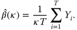
The maximum likelihood estimator of ![]() is the maximizer of
is the maximizer of ![]() over
over ![]() . The maximum likelihood estimator of
. The maximum likelihood estimator of ![]() is
is ![]() .
.
3.4.2.4 The Generalized Pareto Distributions
The one-parameter Pareto distributions were defined in (3.73) and (3.72). We define the two-parameter generalized Pareto distributions, which contain the exponential distributions as a limiting case.
The density functions, distribution functions, and quantile functions have a closed form expression but the maximum likelihood estimator does not have a closed form expression.
The density functions of the generalized Pareto distributions are

where ![]() and
and ![]() . The distribution functions are
. The distribution functions are

The quantile functions are

When ![]() , then the distributions are exponential distributions, defined in (3.65).
, then the distributions are exponential distributions, defined in (3.65).
The generalized Pareto distribution can be defined for the cases ![]() . In this case the support is
. In this case the support is ![]() . See (3.101) for the distribution function and (8.65) for the density function. The generalized Pareto distributions are obtained as limit distributions for threshold exceedances (see Section 3.5.2).
. See (3.101) for the distribution function and (8.65) for the density function. The generalized Pareto distributions are obtained as limit distributions for threshold exceedances (see Section 3.5.2).
For the calculation of the maximum likelihood estimation it is convenient to use the following parameterization. We define the class of generalized Pareto distributions using the tail index ![]() (shape parameter) and the scaling parameter
(shape parameter) and the scaling parameter ![]() by defining the density function as
by defining the density function as
The parameters of the generalized Pareto distribution (3.84) are related to the parameterization in (3.83) by ![]() and
and ![]() . Note that the densities (3.84) can be obtained heuristically from a translation of the one-parameter Pareto distributions, as written in (3.74).
. Note that the densities (3.84) can be obtained heuristically from a translation of the one-parameter Pareto distributions, as written in (3.74).
The maximum likelihood estimator cannot be expressed in a closed form but we can reduce the numerical maximization of the two-variate likelihood function to the numerical maximization of a univariate function. For the computation of the maximum likelihood estimator, we use the parameterization of the density as in (3.84).
The logarithmic likelihood function for i.i.d. observations ![]() is
is

Setting the partial derivative equal to zero and solving for ![]() gives24
gives24

The maximum likelihood estimator ![]() for
for ![]() is the maximizer of the univariate function
is the maximizer of the univariate function ![]() over
over ![]() . The maximum likelihood estimator for
. The maximum likelihood estimator for ![]() is
is ![]() . The maximum likelihood estimators for
. The maximum likelihood estimators for ![]() and
and ![]() are
are
3.4.2.5 The Weibull Distributions
For the Weibull distributions the density functions, distribution functions, and quantile functions have a closed form expression but the maximum likelihood estimator cannot be written in a closed form.
The Weibull densities are defined as

where ![]() is the shape parameter and
is the shape parameter and ![]() is the scale parameter. The distribution function is
is the scale parameter. The distribution function is

The quantile function is
For ![]() we obtain the exponential distribution. The Weibull distributions are also called stretched exponential distributions because
we obtain the exponential distribution. The Weibull distributions are also called stretched exponential distributions because ![]() is a stretched exponential function.
is a stretched exponential function.
The maximum likelihood estimator cannot be expressed in a closed form but we can reduce the numerical maximization of the two-variate likelihood function to the numerical maximization of a univariate function. The logarithmic likelihood function for i.i.d. observations ![]() is
is

Setting the partial derivative equal to zero and solving for ![]() gives25
gives25

The maximum likelihood estimator ![]() for
for ![]() is the maximizer of the univariate function
is the maximizer of the univariate function ![]() over
over ![]() . The maximum likelihood estimator for
. The maximum likelihood estimator for ![]() is
is ![]() .
.
3.4.2.6 A Three Parameter Family
A flexible family for the modeling of the right tail is defined in Malevergne and Sornette (2005, p. 57) by density functions
where ![]() is the starting point of the distribution,
is the starting point of the distribution, ![]() , and
, and ![]() . When
. When ![]() , then
, then ![]() . The normalization constant
. The normalization constant ![]() has the expression
has the expression

where ![]() is the nonnormalized incomplete Gamma function.
is the nonnormalized incomplete Gamma function.
The family contains several sub-families:
- 1. The exponential density is obtained when
 ,
,  ,
,  , and
, and  . The exponential densities are
 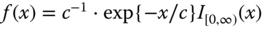 , where
  . We defined exponential densities in (3.65).
 - 2. The Pareto density is obtained when
 and
and  . The Pareto densities are
  , where
  and
and  . We defined Pareto densities in (3.72).
 - 3. The gamma density is obtained by choosing
 and
and  . The gamma densities are
  , where
  and
and  . The gamma densities were defined in (3.80).
 - 4. The Weibull density is obtained when
 ,
,  , and
, and  :
:

- where
 . The Weibull densities were defined in (3.86).
 - 5. The incomplete gamma density is obtained when
 and
and  :
:

- where
 .
.
The Pareto density and the stretched exponential density can be interpolated smoothly by the log-Weibull density
where ![]() .
.
3.4.3 Fitting the Models to Return Data
We fit models first to S&P 500 returns, and then to a collection of individual stocks in S&P 500. Fitting of the distributions gives background for the quantile estimation of Chapter 8.
3.4.3.1 S&P 500 Daily Returns: Maximum Likelihood
We fit one-parameter models (exponential and Pareto) and two-parameter models (gamma, generalized Pareto, and Weibull) to the tails of S&P 500 daily returns. The S&P 500 daily data is described in Section 2.4.1.
We study maximum likelihood estimators (3.63) and (3.64). The estimates are constructed using data
for the left and the right tails, respectively. Threshold ![]() is the
is the ![]() th empirical quantile, and
th empirical quantile, and ![]() is the
is the ![]() th empirical quantile, where
th empirical quantile, where ![]() . The estimators
. The estimators ![]() and
and ![]() depend on the parameter
depend on the parameter ![]() .
.
To show the sensitiveness of the estimates with respect the parameter ![]() we plot the values of the estimates as a function of
we plot the values of the estimates as a function of ![]() . These plots are related to the Hill's plot, which name is used in the case of estimating parameter
. These plots are related to the Hill's plot, which name is used in the case of estimating parameter ![]() of the Pareto distribution.
of the Pareto distribution.
To characterize the goodness of fit we show tail plots, as defined in Section 3.2.1. The tail plots include both the observations and the fitted curves, for several values of ![]() .
.
The one-parameter models indicate that the left tail is heavier than the right tail. However, the two-parameter families seem to give much better fits than the one-parameter families.
The Exponential Model
The maximum likelihood estimator of the parameter of the exponential distribution is given in (3.67). The estimators for the parameters of the left tail and the right tail are obtained from (3.63) and (3.64) as
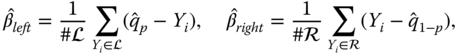
where ![]() and
and ![]() are defined in (3.61) and (3.62). The estimates
are defined in (3.61) and (3.62). The estimates ![]() and
and ![]() are related to the estimates of the expected shortfall in (3.28) and (3.27).
are related to the estimates of the expected shortfall in (3.28) and (3.27).
Figure 3.17 shows estimates of the parameter ![]() and
and ![]() of the exponential distribution. Panel (a) shows estimates of
of the exponential distribution. Panel (a) shows estimates of ![]() and panel (b) shows estimates of
and panel (b) shows estimates of ![]() , as a function of
, as a function of ![]() . Parameter
. Parameter ![]() occurs in the quantile function, and is more important in quantile estimation, but for the convenience of the reader we also show the estimates of the rate parameter
occurs in the quantile function, and is more important in quantile estimation, but for the convenience of the reader we also show the estimates of the rate parameter ![]() . The red curves show the maximum likelihood estimates for the left tail, and the blue curves show the maximum likelihood estimates for the right tail. In addition, we show the values of the regression estimates (3.69) and (3.71). The pink curves show the regression estimates for the left tail, and the green curves show the regression estimates for the right tail. We see that the estimates for
. The red curves show the maximum likelihood estimates for the left tail, and the blue curves show the maximum likelihood estimates for the right tail. In addition, we show the values of the regression estimates (3.69) and (3.71). The pink curves show the regression estimates for the left tail, and the green curves show the regression estimates for the right tail. We see that the estimates for ![]() are larger for the left tail than for the right tail. This indicates that the left tail is heavier than the right tail. The estimates become smaller when
are larger for the left tail than for the right tail. This indicates that the left tail is heavier than the right tail. The estimates become smaller when ![]() increases. The regression estimates are larger than the maximum likelihood estimates. For the estimates of
increases. The regression estimates are larger than the maximum likelihood estimates. For the estimates of ![]() the behavior is opposite.
the behavior is opposite.

Figure 3.17 Exponential model for S&P 500 daily returns: Parameter estimates. Panel (a) shows estimates of  and panel (b) shows estimates of
  , as a function of
  . Red and blue: the maximum likelihood estimates; pink and green: the regression estimates; red and pink: the left tail; blue and green: the right tail.
Figure 3.18 shows tail plots, defined in Section 3.2.1. Panel (a) shows the left tail plots and panel (b) shows the right tail plots. The red and green points show the observed data and the black lines show the exponential distribution functions when parameter ![]() is estimated with maximum likelihood. The four black curves show the cases
is estimated with maximum likelihood. The four black curves show the cases ![]() ,
, ![]() ,
, ![]() , and
, and ![]() . The tails are fitted better with small values of
. The tails are fitted better with small values of ![]() .
.

Figure 3.18 Exponential model for S&P 500 daily returns: Tail plots with maximum likelihood. Panel (a) shows the left tail plots and panel (b) shows the right tail plots. The red and green points show the observed data and the black lines show the exponential fits with  ,
,  ,
,  , and
, and  .
.
The Pareto Model
The maximum likelihood estimator of the parameter of the Pareto distribution is given in (3.75).26 The estimators for the parameters of the left and the right tails are obtained from (3.63) and (3.64) as

where ![]() with
with ![]() for the left tail, and
for the left tail, and ![]() with
with ![]() for the right tail. Now
for the right tail. Now ![]() . The maximum likelihood estimators are called Hill's estimators.27
. The maximum likelihood estimators are called Hill's estimators.27
Figure 3.19 shows estimates of the parameter ![]() and
and ![]() of the Pareto distribution. Panel (a) shows estimates of
of the Pareto distribution. Panel (a) shows estimates of ![]() and panel (b) shows estimates of
and panel (b) shows estimates of ![]() , as a function of
, as a function of ![]() . The plot in panel (b) is known as Hill's plot. Parameter
. The plot in panel (b) is known as Hill's plot. Parameter ![]() occurs in the quantile function, and is more important in quantile estimation, but for the convenience of the reader we also show the estimates of parameter
occurs in the quantile function, and is more important in quantile estimation, but for the convenience of the reader we also show the estimates of parameter ![]() . The red curves show the maximum likelihood estimates for the left tail and the blue curves show the maximum likelihood estimates for the right tail. In addition, we show the values of regression estimates of
. The red curves show the maximum likelihood estimates for the left tail and the blue curves show the maximum likelihood estimates for the right tail. In addition, we show the values of regression estimates of ![]() , defined in (3.76), and the values of regression estimates of
, defined in (3.76), and the values of regression estimates of ![]() , defined in (3.77). The pink curves show the regression estimates for the left tail and the green curves show the regression estimates for the right tail. We see that the estimates of
, defined in (3.77). The pink curves show the regression estimates for the left tail and the green curves show the regression estimates for the right tail. We see that the estimates of ![]() are larger for the left tail than for the right tail, which means that the left tail is estimated to be heavier than the right tail. The estimates of
are larger for the left tail than for the right tail, which means that the left tail is estimated to be heavier than the right tail. The estimates of ![]() become larger when
become larger when ![]() increases. The regression estimates of
increases. The regression estimates of ![]() are smaller than the maximum likelihood estimates. For the estimates of
are smaller than the maximum likelihood estimates. For the estimates of ![]() the behavior is opposite.
the behavior is opposite.

Figure 3.19 Pareto model for S&P 500 daily returns: Parameter estimates. Panel (a) shows estimates of  and panel (b) shows estimates of
  as a function of
  . Red and blue: the maximum likelihood estimates; pink and green: the regression estimates; red and pink: the left tail; blue and green: the right tail.
Figure 3.20 shows tail plots. Panel (a) shows the left tail plots and panel (b) shows the right tail plots. The red and green points show the observed data and the black curves show the Pareto distribution functions when parameter ![]() is estimated with maximum likelihood. The four black curves show the cases
is estimated with maximum likelihood. The four black curves show the cases ![]() ,
, ![]() ,
, ![]() , and
, and ![]() .
.

Figure 3.20 Pareto model for S&P 500 daily returns: Tail plots with maximum likelihood. Panel (a) shows the left tail plots and panel (b) shows the right tail plots. The red and green points show the observed data and the black curves show the fits with  ,
,  ,
,  , and
, and  .
.
The Gamma Model
The gamma densities are defined in (3.80). The maximum likelihood estimators for the scale parameter ![]() and for the shape parameter
and for the shape parameter ![]() of a gamma distribution do not have a closed form expression, but the computation can be done by minimizing a univariate function. We get the maximum likelihood estimates for the parameters of the left tail and the right tail by applying the numerical procedure for the observations
of a gamma distribution do not have a closed form expression, but the computation can be done by minimizing a univariate function. We get the maximum likelihood estimates for the parameters of the left tail and the right tail by applying the numerical procedure for the observations
for the left and the right tails, respectively, where ![]() .
.
Figure 3.21(a) shows estimates of ![]() and panel (b) shows estimates of
and panel (b) shows estimates of ![]() . The red curves show the estimates for the left tail, and the blue curves show the estimates for the right tail. We see that the estimates for
. The red curves show the estimates for the left tail, and the blue curves show the estimates for the right tail. We see that the estimates for ![]() are larger for the left tail than for the right tail. The estimates become smaller when
are larger for the left tail than for the right tail. The estimates become smaller when ![]() increases.
increases.

Figure 3.21 Gamma model for S&P 500 daily returns: Parameter estimates. Panel (a) shows estimates of  and panel (b) shows estimates of
  , as a function of
  . Red: the left tail; blue: the right tail.
Figure 3.22 shows tail plots. Panel (a) shows the left tail plots and panel (b) shows the right tail plots. The red and green points show the observed data and the black curves show the gamma distribution functions when parameters are estimated with maximum likelihood. The four black curves show the cases ![]() ,
, ![]() ,
, ![]() , and
, and ![]() .
.

Figure 3.22 Gamma model for S&P 500 daily returns: Tail plots with maximum likelihood. Panel (a) shows the left tail plots and panel (b) shows the right tail plots. The red and green points show the observed data and the black lines show the fits with  ,
,  ,
,  , and
, and  .
.
The Generalized Pareto Model
The density of a generalized Pareto distribution is given in (3.82). The maximum likelihood estimators for the scale parameter ![]() and for the shape parameter
and for the shape parameter ![]() of a generalized Pareto distribution do not have a closed form expression, but the computation can be done by minimizing a univariate function. We get the maximum likelihood estimates for the parameters of the left tail and the right tail by applying the numerical procedure for the observations in (3.92).
of a generalized Pareto distribution do not have a closed form expression, but the computation can be done by minimizing a univariate function. We get the maximum likelihood estimates for the parameters of the left tail and the right tail by applying the numerical procedure for the observations in (3.92).
Figure 3.23(a) shows estimates of ![]() , and panel (b) shows estimates of
, and panel (b) shows estimates of ![]() . The red curves show the estimates for the left tail, and the blue curves show the estimates for the right tail. The estimates of
. The red curves show the estimates for the left tail, and the blue curves show the estimates for the right tail. The estimates of ![]() become smaller when
become smaller when ![]() increases.
increases.
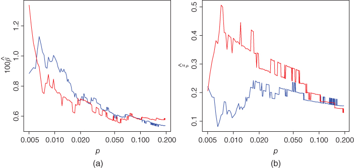
Figure 3.23 Generalized Pareto model for S&P 500 daily returns: Parameter estimates. Panel (a) shows estimates of  and panel (b) shows estimates of
  , as a function of
  . Red shows the estimates for the left tail, and blue shows them for the right tail.
Figure 3.24 shows tail plots. Panel (a) shows the left tail plots and panel (b) shows the right tail plots. The red and green points show the observed data and the black curves show the distribution functions when parameters are estimated using maximum likelihood. The four black curves show the cases ![]() ,
, ![]() ,
, ![]() , and
, and ![]() . The fitted curves do not change in a monotonic order when
. The fitted curves do not change in a monotonic order when ![]() is decreased.
is decreased.

Figure 3.24 Generalized Pareto model for S&P 500 daily returns: Tail plots with maximum likelihood. Panel (a) shows the left tail plots and panel (b) shows the right tail plots. The red and green points show the observed data and the black curves show the fits with  ,
,  ,
,  , and
, and  .
.
The Weibull Model
The Weibull densities are given in (3.86). The maximum likelihood estimators for the scale parameter ![]() and for the shape parameter
and for the shape parameter ![]() of a Weibull distribution do not have a closed form expression, but the computation can be done by minimizing a univariate function. We get the maximum likelihood estimates for the parameters of the left tail and the right tail by applying the numerical procedure for the observations in (3.92).
of a Weibull distribution do not have a closed form expression, but the computation can be done by minimizing a univariate function. We get the maximum likelihood estimates for the parameters of the left tail and the right tail by applying the numerical procedure for the observations in (3.92).
Figure 3.25(a) shows estimates of ![]() , and panel (b) shows estimates of
, and panel (b) shows estimates of ![]() . The red curves show the estimates for the left tail, and the blue curves show the estimates for the right tail. The estimates of
. The red curves show the estimates for the left tail, and the blue curves show the estimates for the right tail. The estimates of ![]() become smaller when
become smaller when ![]() increases.
increases.

Figure 3.25 Weibull model for S&P 500 daily returns: Parameter estimates. Panel (a) shows estimates of  and panel (b) shows estimates of
  , as a function of
  . Red shows the estimates for the left tail, and blue shows them for the right tail.
Figure 3.26 shows tail plots. Panel (a) shows the left tail plots and panel (b) shows the right tail plots. The red and green points show the observed data and the black curves show the distribution functions when parameters are estimated using maximum likelihood. The four black curves show the cases ![]() ,
, ![]() ,
, ![]() , and
, and ![]() .
.

Figure 3.26 Weibull model for S&P 500 daily returns: Tail plots with maximum likelihood. Panel (a) shows the left tail plots and panel (b) shows the right tail plots. The red and green points show the observed data and the black curves show the fits with  ,
,  ,
,  , and
, and  .
.
3.4.3.2 Tail Index Estimation for S&P 500 Components
We study fitting of the Pareto model for the daily returns of stocks in S&P 500 index. S&P 500 components data is described in Section 2.4.5.
Figure 3.27 shows how ![]() and
and ![]() are distributed. The estimators are defined in (3.89); these are Hill's estimators for the left and right Pareto indexes. Panel (a) shows the distribution of the estimates of the left tail index and panel (b) shows the distribution of the estimates of the right tail index. We have computed the estimates for each 312 stocks in the S&P 500 components data set, and the kernel density estimator is applied for this data set of 312 observations. This is done for
are distributed. The estimators are defined in (3.89); these are Hill's estimators for the left and right Pareto indexes. Panel (a) shows the distribution of the estimates of the left tail index and panel (b) shows the distribution of the estimates of the right tail index. We have computed the estimates for each 312 stocks in the S&P 500 components data set, and the kernel density estimator is applied for this data set of 312 observations. This is done for ![]() . The smoothing parameter is chosen by the normal reference rule, and the standard Gaussian kernel function is used. A smaller
. The smoothing parameter is chosen by the normal reference rule, and the standard Gaussian kernel function is used. A smaller ![]() gives a smaller estimate of
gives a smaller estimate of ![]() .
.

Figure 3.27 Density estimates of the distribution of Hill's estimates. (a) Distribution of the left tail index; (b) the right tail index. Hill's estimates are calculated for the 312 stocks and kernel estimates are calculated from 312 estimated values of  . There is an kernel estimate for each
  .
.
Figure 3.28 shows a scatter plot of points ![]() , when the estimates are computed for each stock in the S&P 500 components data. We have used
, when the estimates are computed for each stock in the S&P 500 components data. We have used ![]() . There are about the same number of stocks for which the left tail index is smaller than the right tail index
. There are about the same number of stocks for which the left tail index is smaller than the right tail index

Figure 3.28 A scatter plot of estimates of  . We show a scatter plot of points
  for the stocks in the S&P 500 components data. The red line shows the points with
  .
.
3.5 Asymptotic Distributions
First we describe central limit theorems and second we describe limit theorems for the excess distribution. The limit distributions of the central limit theorems can be used to model the complete return distribution of a financial asset and the limit distributions for the excess distribution can be used to model the tail areas of the return distribution of a financial asset.
3.5.1 The Central Limit Theorems
We applied a central limit theorem for sums in (3.46) and (3.49) to justify the normal and the log-normal model for the stock prices. In a similar way we can apply the central limit theorems to justify alternative models for the stock prices. When the variance of the summands is finite the limit is a normal distribution, but if the variance is not finite, the limit distributions can have heavier tails than the normal distributions.
We describe first a central limit theorem for sums of independent but not necessarily identically distributed random variables. The limit distributions belong to the class of infinitely divisible distributions. Second we describe central limit theorems for sums of independent and identically distributed random variables. Now the limit distributions belong to the class of stable distributions. The class of stable distributions is a subset of the class of infinitely divisible distributions. The stable distributions include the normal distributions but they include also heavy tailed distributions, which can be used to describe phenomena where both very large and very small values can be observed, like the stock returns.
Third we consider the case of sums of dependent random variables. When the dependence is weak, then a convergence towards a normal distribution occurs, but the asymptotic variance is affected by the dependence.
We do not apply stable distributions or infinitely divisible distributions to model return distributions, but it is useful to note that heavy tailed distributions arise already from central limit theorems, and not only from limit distributions for the excess distribution.
3.5.1.1 Sums of Independent Random Variables
The Khintchine theorem states that for a distribution to be a limit distribution of a sum of independent (but not necessarily identically distributed) random variables it is necessary and sufficient that the distribution is infinitely divisible; see Billingsley (2005, pp. 373–374) and Breiman (1993, p. 191).
The infinitely divisible distributions are such that a random variable following an infinitely divisible distribution can be represented as a sum of ![]() i.i.d. random variables for each natural number
i.i.d. random variables for each natural number ![]() . In other words, a distribution function
. In other words, a distribution function ![]() is infinitely divisible if for each
is infinitely divisible if for each ![]() there is a distribution function
there is a distribution function ![]() such that
such that ![]() is the
is the ![]() -fold convolution
-fold convolution ![]() .28 For example, the normal, Poisson, and gamma distributions are infinitely divisible but the uniform distributions are not. See Billingsley (2005, Chapter 5) and Breiman (1993, Section 9.5) about infinitely divisible distributions.
.28 For example, the normal, Poisson, and gamma distributions are infinitely divisible but the uniform distributions are not. See Billingsley (2005, Chapter 5) and Breiman (1993, Section 9.5) about infinitely divisible distributions.
Let ![]() ,
, ![]() , be a triangular array of row-wise independent random variables which satisfy
, be a triangular array of row-wise independent random variables which satisfy
as ![]() , for every
, for every ![]() . Then
. Then ![]() can be normalized to converge to an infinitely divisible distribution.
can be normalized to converge to an infinitely divisible distribution.
3.5.1.2 Sums of Independent and Identically Distributed Random Variables
For a distribution to be a limit distribution of a sum of independent and identically distributed random variables it is necessary and sufficient that the distribution is stable.
Stable Distributions
A random variable is said to have a stable distribution, if for every natural number ![]() and for
and for ![]() independent and with the same distribution as
independent and with the same distribution as ![]() , there are constants
, there are constants ![]() and
and ![]() such that
such that
holds in distribution; see Breiman (1993, p. 199). Stable distributions are infinitely divisible distributions, because the distribution function of ![]() is the
is the ![]() -fold convolution of
-fold convolution of ![]() , where
, where ![]() is the distribution function of
is the distribution function of ![]() . In particular, the sum of two independent and identically distributed stable random variables has also a stable distribution.
. In particular, the sum of two independent and identically distributed stable random variables has also a stable distribution.
Density functions of stable distributions cannot be written in a closed form in general. The characteristic function of a stable distribution is

where

Note that ![]() is the sign of
is the sign of ![]() , and we can define
, and we can define ![]() . Parameter
. Parameter ![]() is the exponent of the distribution, which is related to the heaviness of the tails,
is the exponent of the distribution, which is related to the heaviness of the tails, ![]() is the location term,
is the location term, ![]() is the scale factor, and
is the scale factor, and ![]() is the asymmetry parameter (skewness parameter). When
is the asymmetry parameter (skewness parameter). When ![]() , then distribution is symmetric, when
, then distribution is symmetric, when ![]() , then distribution is skewed to the right, and when
, then distribution is skewed to the right, and when ![]() , the distribution is skewed to the left. See Breiman (1993, p. 204).
, the distribution is skewed to the left. See Breiman (1993, p. 204).
The analytical form of the density is known for ![]() (Gaussian),
(Gaussian), ![]() ,
, ![]() (Cauchy), and
(Cauchy), and ![]() ,
, ![]() (Lévy–Smirnov or Lévy). The density of the Cauchy distribution is given by
(Lévy–Smirnov or Lévy). The density of the Cauchy distribution is given by
The Cauchy distribution is the Student distribution for the degrees of freedom ![]() . The density of the Lévy–Smirnov distribution is given by
. The density of the Lévy–Smirnov distribution is given by

Symmetric stable distributions are stable distributions with location parameter ![]() and skewness parameter
and skewness parameter ![]() . The characteristic function of a symmetric stable distribution is
. The characteristic function of a symmetric stable distribution is
where ![]() and
and ![]() . The density of a symmetric stable distribution can be written as a series expansion
. The density of a symmetric stable distribution can be written as a series expansion

where ![]() is defined through
is defined through

Symmetric stable distributions have the power-law behavior of the tails:

Equation (3.94) gives the leading asymptotic term in (3.93). For the distributions with Pareto tails the ![]() th moment does not exist if
th moment does not exist if ![]() . This implies that the variance of a symmetric stable distribution is always infinite, and the mean is infinite when
. This implies that the variance of a symmetric stable distribution is always infinite, and the mean is infinite when ![]() . The mode is used as the location parameter of the symmetric stable distributions (symmetric stable distributions are unimodal).
. The mode is used as the location parameter of the symmetric stable distributions (symmetric stable distributions are unimodal).
Convergence to a Stable Distribution
The central limit theorems were presented in Gnedenko and Kolmogorov (1954), Feller (1957), and Feller (1966). We follow the exposition of Embrechts et al. (1997, Theorem 2.2.15). Assume that ![]() are independent and identically distributed with the same distribution as
are independent and identically distributed with the same distribution as ![]() .
.
- 1. Assume that
 . Then,

- where
 and
and  .
. - 2. Assume that

- is slowly varying.29
- Let
 be the solution of the equation
- where

- Then,

- where
 . It holds that
 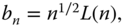 for a slowly varying function
  .
. - 3. Assume that the distribution function
 of
of  satisfies

- as
 , where
  is slowly varying, and
  ,
,  . Let
. Let  be the solution of (3.95). Then,

- where
 and
and  is a stable distribution with
  .
.
3.5.1.3 Sums of Dependent Random Variables
We apply a limit theorem for dependent random variables in Sections 6.2.2 and 10.1.2.
Let ![]() be a strictly stationary time series. We define the weak dependence in terms of a condition on the
be a strictly stationary time series. We define the weak dependence in terms of a condition on the ![]() -mixing coefficients. Let
-mixing coefficients. Let ![]() denote the sigma algebra generated by random variables
denote the sigma algebra generated by random variables ![]() . The
. The ![]() -mixing coefficient is defined as
-mixing coefficient is defined as
where ![]() . Now we can state the central limit theorem. Let
. Now we can state the central limit theorem. Let ![]() and
and ![]() for some constant
for some constant ![]() . Then,
. Then,

where

![]() , and we assume that
, and we assume that ![]() . Ibragimov and Linnik (1971, Theorem 18.4.1) gave necessary and sufficient conditions for a central limit theorem under
. Ibragimov and Linnik (1971, Theorem 18.4.1) gave necessary and sufficient conditions for a central limit theorem under ![]() -mixing conditions. A proof for our statement of the central limit theorem in (3.96) can be found in Peligrad (1986); see also Fan and Yao (2005, Theorem 2.21) and Billingsley (2005, Theorem 27.4).
-mixing conditions. A proof for our statement of the central limit theorem in (3.96) can be found in Peligrad (1986); see also Fan and Yao (2005, Theorem 2.21) and Billingsley (2005, Theorem 27.4).
3.5.2 The Limit Theorems for Maxima
Since we have modeled the excess distribution parametrically, it is of special interest that the limit distribution of the excess distribution is a generalized Pareto distribution; this limit theorem is stated in (3.102). The weak convergence of maxima is related to the convergence of the excess distribution.
3.5.2.1 Weak Convergence of Maxima
Let the real valued random variables ![]() be independent and identically distributed, and denote the maximum
be independent and identically distributed, and denote the maximum
Sometimes convergence in distribution holds in the sense that there exists sequences ![]() and
and ![]() where
where ![]() and
and ![]() so that
so that

for all ![]() , as
, as ![]() , where
, where ![]() is a distribution function,
is a distribution function, ![]() , and
, and ![]() . The Fisher–Tippett–Gnedenko theorem states that if the convergence in (3.97) holds, then
. The Fisher–Tippett–Gnedenko theorem states that if the convergence in (3.97) holds, then ![]() can only be a Fréchet, Weibull, or Gumbel distribution function. See Fisher and Tippett (1928), Gnedenko (1943), and Embrechts et al. (1997, p. 121).
can only be a Fréchet, Weibull, or Gumbel distribution function. See Fisher and Tippett (1928), Gnedenko (1943), and Embrechts et al. (1997, p. 121).
To derive the result for the minimum we use the fact that for
we have ![]() . Let us denote
. Let us denote
so that ![]() . Now,
. Now,
3.5.2.2 Extreme Value Distributions
The Fréchet distribution functions are

where ![]() . The Weibull distribution functions are
. The Weibull distribution functions are

where ![]() . The Gumbel distribution function is
. The Gumbel distribution function is
These distributions are called the extreme value distributions.
Define

Then,

where ![]() is defined on set
is defined on set ![]() . This is known as the Jenkinson–von Mises representation of the extreme value distributions, or the generalized extreme value distribution; see Embrechts et al. (1997, p. 152). We obtain the parametric class of possible limit distributions
. This is known as the Jenkinson–von Mises representation of the extreme value distributions, or the generalized extreme value distribution; see Embrechts et al. (1997, p. 152). We obtain the parametric class of possible limit distributions
where ![]() is the shape parameter,
is the shape parameter, ![]() , and
, and ![]() . The support of the distribution is
. The support of the distribution is ![]() .
.
Using (3.98), we obtain the class of limit distribution functions for the minima. The limit distribution functions are
where ![]() ,
, ![]() ,
, ![]() , and
, and ![]() . Distribution function
. Distribution function ![]() is defined on set
is defined on set ![]() .
.
3.5.2.3 Convergence to an Extreme Value Distribution
If the distribution that generated the observations ![]() has polynomial tails, then (3.97) holds and the limit distribution of the maximum belongs to the Fréchet class. More precisely, if
has polynomial tails, then (3.97) holds and the limit distribution of the maximum belongs to the Fréchet class. More precisely, if
for some slowly varying function ![]() , then a normalized maximum converges to a Fréchet distribution
, then a normalized maximum converges to a Fréchet distribution ![]() ; see Embrechts et al. (1997, p. 131).
; see Embrechts et al. (1997, p. 131).
Let ![]() be the endpoint of the distribution of
be the endpoint of the distribution of ![]() . If
. If ![]() and
and
for some slowly varying function ![]() , then a normalized maximum converges to a Weibull distribution
, then a normalized maximum converges to a Weibull distribution ![]() ; see Embrechts et al. (1997, p. 135). The equation
; see Embrechts et al. (1997, p. 135). The equation
explains the relation between the convergence to a Fréchet distribution and to a Weibull distribution.
If the distribution which generated the observations is exponential, normal, or log-normal, then (3.97) holds and the limit distribution of the maximum is the Gumbel distribution. See Embrechts et al. (1997, p. 145).
3.5.2.4 Generalized Pareto Distributions
The distribution function of the generalized Pareto distribution is

where ![]() . When
. When ![]() , then
, then ![]() . When
. When ![]() , then
, then ![]() . When
. When ![]() , then the distributions are exponential distributions. Note that
, then the distributions are exponential distributions. Note that
where ![]() is the distribution function of a generalized extreme value distribution, as defined in (3.100). Parameter
is the distribution function of a generalized extreme value distribution, as defined in (3.100). Parameter ![]() is a shape parameter and parameter
is a shape parameter and parameter ![]() is a scale parameter. The Pareto distributions were defined in (3.73) and (3.83).
is a scale parameter. The Pareto distributions were defined in (3.73) and (3.83).
3.5.2.5 Convergence to a Generalized Pareto Distribution
Let ![]() be a random variable and let
be a random variable and let ![]() be the distribution function of
be the distribution function of ![]() . We define the excess distribution with threshold
. We define the excess distribution with threshold ![]() as the distribution with the distribution function
as the distribution with the distribution function

We can typically approximate the distribution function ![]() with the distribution function of a generalized Pareto distribution. This follows from the Gnedenko–Pickands–Balkema–de Haan theorem; see Embrechts et al. (1997, p. 158). Let
with the distribution function of a generalized Pareto distribution. This follows from the Gnedenko–Pickands–Balkema–de Haan theorem; see Embrechts et al. (1997, p. 158). Let ![]() . The Gnedenko–Pickands–Balkema–de Haan theorem states that
. The Gnedenko–Pickands–Balkema–de Haan theorem states that
for some positive function ![]() if and only if
if and only if ![]() belongs to the maximum domain of attraction of
belongs to the maximum domain of attraction of ![]() , where
, where ![]() . To say that
. To say that ![]() belongs to the maximum domain of attraction of
belongs to the maximum domain of attraction of ![]() means that (3.97) holds for some sequences
means that (3.97) holds for some sequences ![]() and
and ![]() .
.
The basic idea of deriving the limit distribution of the excess distribution from the limit distribution of the maximum comes from the Poisson approximation. The Poisson approximation states that
and
are equivalent, where ![]() ,
, ![]() is a sequence of real numbers, and
is a sequence of real numbers, and ![]() is the maximum of i.i.d. random variables; see Embrechts et al. (1997, p. 116).30
is the maximum of i.i.d. random variables; see Embrechts et al. (1997, p. 116).30
When the distribution function of the maximum ![]() can be approximated by
can be approximated by

for some ![]() and
and ![]() , then
, then ![]() can be approximated by the distribution function
can be approximated by the distribution function

defined on set ![]() , where
, where

Figure 3.29 Simulated i.i.d. time series. We have simulated 10,000 observations. (a) Student's  -distribution with degrees of freedom
  ; (b) Student's
  -distribution with degrees of freedom
  ; (c) Gaussian distribution. The mean of the observations is zero and the standard deviation is equal to the standard deviation of the S&P 500 returns.
3.6 Univariate Stylized Facts
The heaviness of the tails is one of the main univariate stylized facts. There are several questions related to the heaviness of the tails. We give a list of the observations that can be obtained from the figures of this chapter, and give some references to the literature.
- 1. How heavy are the tails of S&P 500 returns?
Figure 2.1(b) shows a time series of S&P 500 daily returns. To highlight the heaviness of the tails we can compare the real time series with the simulated time series in Figure 3.29. Panel (a) shows uncorrelated observations whose distribution is the
 -distribution with three degrees of freedom, in panel (b) the
  -distribution has six degrees of freedom, and in panel (c) the distribution of the observations is Gaussian.31
Figure 3.2 shows tail plots of S&P 500 daily returns:
 -distribution with degrees of freedom three and four gives reasonable fits both for the left tail and the right tails.
Figure 3.4 shows exponential regression plots of S&P 500 daily returns: The tails seem to be heavier than the exponential tails.
Figure 3.5 shows exponential regression plots of S&P 500 daily returns, and fits both exponential and Pareto distributions: Pareto fits seem to be better.
Figure 3.6 shows Pareto regression plots of S&P 500 daily returns: The tails seem to fit reasonably well for the Pareto model.
Figure 3.7 shows Pareto regression plots of S&P 500 daily returns, and fits both exponential and Pareto distributions: Pareto fits seem to be better.
Figure 3.13 shows how estimates of parameters
 and
and  of Student distribution for S&P 500 components are distributed: The mode of
  is about 3.5 and the range of values of the estimates is about
  .
.Figure 3.27 shows kernel density estimates of the distribution of the estimates of Pareto left tail index and Pareto right tail index for S&P 500 components: The choice of parameter
 has a significant influence on the value of the estimate, but we are in the range
  .
. - 2. How the heaviness of the tails varies across asset classes (stocks, bonds, indexes)?
Figure 2.5(b) shows a times series of US 10-year bond monthly returns. The time series can be compared to the times series of S&P 500 daily returns in Figure 2.1(b), or to the simulated time series in Figure 3.29.
Figure 3.1 shows empirical distribution functions of S&P 500 and US 10-year bond monthly returns: S&P 500 seems to have heavier tails than 10-year bond.
Figure 3.3 shows smooth tail plots of the daily returns of S&P 500 components and of S&P 500 index: The individual components seem to have heavier tails than the index.
Figure 3.8 shows empirical quantile functions of S&P 500 and US 10-year bond monthly returns: S&P 500 seems to have heavier tails than 10-year bond.
Figure 3.10(a) shows kernel density estimates of S&P 500 and US 10-year bond monthly returns: These estimates do not reveal information about the tails, but in the central area 10-year bond seems to be more concentrated around zero than S&P 500. Cont (2001) reports that returns of US Treasury bonds are positively skewed, whereas the returns of stock indices are negatively skewed.
Bouchaud (2002) reports that the tails of the stock returns have Pareto (power-law) tails
 , where
  is approximately 3, but emerging markets can have
  smaller than 2. Cont (2001) notes that the tail index varies between 2 and 5 that excludes the Gaussian and the stable laws with infinite variance. The standard deviation of daily returns is 3% for stocks, 1% for stock indices, and 0.03% for short term interest rates; see Bouchaud (2002).
 - 3. What is the best model for the tails?
Figures 3.17–3.26 study fitting of parametric models to the tails of S&P 500 returns. In particular, tail plots are shown for the exponential distribution in Figure 3.18, for the Pareto distribution in Figure 3.20, for the gamma distribution in Figure 3.22, for the generalized Pareto distribution in Figure 3.24, and for the Weibull distribution in Figure 3.26. Two-parameter families give reasonable fits, in particular, the generalized Pareto distribution gives a good fit.
Malevergne and Sornette (2005) give a review of fitting Pareto distributions, stretched exponentials and log-Weibull distributions.
- 4. Are the left tail and the right equally heavy?
The parameter estimates for fitting models to the daily returns of S&P 500 indicate that the left tail is heavier than the right tail (see Figures 3.17, 3.19, 3.21, 3.23, and 3.25).
Figure 3.28 shows values of estimates of Pareto tail index
 for S&P 500 components, both for the left and right tail: There seems to be equal amount of stocks with a larger left tail index as there are stocks with a larger right tail index.
Cont (2001) reports that gains and loss are asymmetric; large drawdowns are observed but not equally large upward movements.
- 5. How the heaviness of the tails is affected by the return horizon?
Figure 3.12 shows values of estimates of parameters of
 -distribution (degrees of freedom
  and scaling parameter
  ) for various return horizons of S&P 500 returns: the estimates increase from
  for daily returns to
  for 2-month returns. Also
  increases with the return horizon.
Figure 3.10(b) shows kernel density estimates of the S&P 500 return distribution when the return horizon varies between one and five days.
Cont (2001) observes that the distribution of returns looks more and more like a Gaussian distribution when the time scale is increased.

when ![]() , where
, where ![]() is the joint density of
is the joint density of ![]() , and
, and ![]() is the density of
is the density of ![]() :
:

If ![]() , then
, then ![]() .
.
The absolute shortfall for the left tail is related to the lower partial moment of order ![]() and target rate
and target rate ![]() :
:
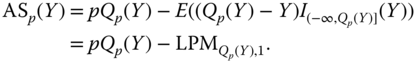
The absolute shortfall is estimated from observations ![]() by
by

where ![]() is the ordered sample and
is the ordered sample and ![]() . Here, we divide by
. Here, we divide by ![]() , but in the estimator (3.28) of the expected shortfall we divide by
, but in the estimator (3.28) of the expected shortfall we divide by ![]() .
.

where ![]() .
.
where ![]() and
and ![]() . Then the histogram can be written as
. Then the histogram can be written as

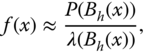
where ![]() ,
, ![]() is small, and
is small, and ![]() is the Lebesgue measure of
is the Lebesgue measure of ![]() . We have that
. We have that

when ![]() . We arrive into (3.43) by allowing other kernel functions than only the indicator function.
. We arrive into (3.43) by allowing other kernel functions than only the indicator function.
where ![]() is the sample variance, when we assume that
is the sample variance, when we assume that ![]() is known. Analogously, in simulations we have to note that when
is known. Analogously, in simulations we have to note that when ![]() , then
, then

has mean ![]() and variance
and variance ![]() .
.

The logarithmic likelihood is

Putting the derivative equal to zero and solving the equation gives the maximum likelihood estimator.

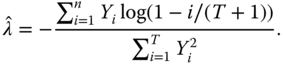

where it is assumed that ![]() are i.i.d. Pareto distributed random variables. Taking logarithms leads to
are i.i.d. Pareto distributed random variables. Taking logarithms leads to
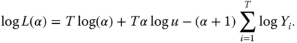
Differentiating with respect to ![]() and setting the derivative equal to zero gives the maximum likelihood estimator.
and setting the derivative equal to zero gives the maximum likelihood estimator.

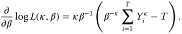

and

if ![]() . Also, because
. Also, because ![]() ,
,
if ![]() . (We can argue that now
. (We can argue that now ![]() .) We have assumed that
.) We have assumed that ![]() .
.