
Chapter 16
Quadratic and Local Quadratic Hedging
Quadratic hedging was introduced in Sections 13.1.3 and 15.1. In quadratic hedging we find the best approximation of the option in the sense of the mean-squared error. Quadratic hedging is related to the idea of statistical arbitrage: The fair price is defined as such price that makes the probability of gains and losses small for the writer of the option.
Quadratic hedging makes it possible to price and hedge options in a completely nonparametric way. In quadratic hedging we can derive prices and hedging coefficients without any modeling assumptions, making only some rather weak assumptions about square integrability and about a bounded mean–variance trade-off. There are many ways to implement quadratic hedging nonparametrically. We use kernel estimation in our implementation.
Let ![]() be the discounted payoff of an European option. For example, for a call option
be the discounted payoff of an European option. For example, for a call option ![]() . In quadratic hedging the mean-squared hedging error
. In quadratic hedging the mean-squared hedging error
is minimized among strategies ![]() and among the initial investment
and among the initial investment ![]() . The terminal value of the gains process is defined by
. The terminal value of the gains process is defined by

where ![]() is the discounted price vector. The problem resembles least-squares linear regression, where
is the discounted price vector. The problem resembles least-squares linear regression, where ![]() is the response variable,
is the response variable, ![]() are the explanatory variables,
are the explanatory variables, ![]() is the intercept, and
is the intercept, and ![]() are the regression coefficients. However, now we have a time series setting, where the “explanatory” variable
are the regression coefficients. However, now we have a time series setting, where the “explanatory” variable ![]() is observed at time
is observed at time ![]() . We can use the knowledge of the observed values of
. We can use the knowledge of the observed values of ![]() in choosing
in choosing ![]() . In the usual linear regression all regression coefficients are chosen at the same time:
. In the usual linear regression all regression coefficients are chosen at the same time: ![]() .
.
Quadratic hedging in discrete time is explained in monographs Föllmer and Schied (2002, p. 393), Bouchaud and Potters (2003), and Černý (2004b). Earlier studies include Föllmer and Schweizer (1989), Bouchaud and Sornette (1994), Schweizer (1994), and Schäl (1994). Early continuous time studies include Föllmer and Sondermann (1986) and Duffie and Richardson (1991).
We study quadratic hedging and pricing in three steps: first for the one period model, then for the two period model, and finally the formulas are given for the general multiperiod model. The multiperiod model contains as special cases the one and two period models, but we think that it is helpful to study the one and two period models separately, because in these models the formulas are more transparent and notationally more convenient than in the multiperiod model. The generalization from the two period model to the multiperiod model is straightforward.
Local quadratic hedging simplifies the minimization problem of quadratic hedging, and it can achieve easier computations. In the one period model quadratic hedging and local quadratic hedging are equivalent, but in the multiperiod models they are different.
The price and the hedging coefficients of quadratic hedging do not have a closed-form expression, but only a recursive definition. This recursive definition can be used in computations, but the implementation is not trivial. We implement only the local quadratic hedging and pricing. We need to estimate various conditional expectations. We estimate the conditional expectations using historical simulation: The time series of previous returns is used to construct a large number of price sequences, and conditional expectations are estimated as sample means over price sequences. The observed volatility is used as the conditioning variable. Separate methods are used for the case of independent and dependent increments.
We evaluate quadratic hedging by studying the distribution of the hedging errors. The distribution should be concentrated around zero as well as possible. The main observation is that even the simplest setting of local quadratic hedging with independent increments leads to a distribution of the hedging errors that is better concentrated around zero than the distribution of the hedging errors when Black–Scholes hedging with GARCH(![]() ) volatility is used.
) volatility is used.
Section 16.1 studies global quadratic hedging and pricing. Section 16.2 studies local quadratic hedging and pricing. Section 16.3 studies implementations of local quadratic hedging.
16.1 Quadratic Hedging
The exact solution for quadratic hedging can be given using backward induction. We present the solution in three steps: first for the one period model, second for the two period model, and third for the general model.
16.1.1 Definitions and Assumptions
We recall the notation from Section 13.2, and in particular from Section 13.2.2. We assume that there is only one risky asset: ![]() . The price process of the riskless bond is denoted by
. The price process of the riskless bond is denoted by ![]() . We choose
. We choose
where ![]() . The notation is a short hand for
. The notation is a short hand for ![]() , where
, where ![]() is the time between two steps, expressed in fractions of a year, and
is the time between two steps, expressed in fractions of a year, and ![]() is the annual interest rate. The time series of prices of the risky asset is denoted by
is the annual interest rate. The time series of prices of the risky asset is denoted by ![]() . The complete price vector is denoted by
. The complete price vector is denoted by
A trading strategy is
where the values ![]() and
and ![]() express the quantity of the bond and the risky asset held between
express the quantity of the bond and the risky asset held between ![]() and
and ![]() .
.
16.1.1.1 Wealth and Value Processes
The wealth at time 0 is ![]() , and after that
, and after that
Under the condition of self-financing the wealth at time ![]() was written in (13.5) as
was written in (13.5) as

where ![]() .
.
The discounted price process is defined by

We denote ![]() . The value process was defined in (13.8) as
. The value process was defined in (13.8) as

Under the condition of self-financing the value at time ![]() can be written as
can be written as

where ![]() .
.
The gains process is defined as

For a self-financing strategy
16.1.1.2 Quadratic Hedging
We use the terms “quadratic hedging” and “global quadratic hedging” to mean the same thing. The term “global quadratic hedging” is used when a distinction to “local quadratic hedging” is emphasized. We use the term “quadratic price” to mean the price that is implied by quadratic hedging.
Let ![]() be the value of an European option. For example,
be the value of an European option. For example, ![]() . Let
. Let ![]() . A quadratic strategy
. A quadratic strategy ![]() is a minimizer of
is a minimizer of
over ![]() and over self-financing strategies
and over self-financing strategies ![]() . We obtain the quadratic price
. We obtain the quadratic price
In the general case the quadratic price is ![]() , but in our case
, but in our case ![]() . The bond coefficients
. The bond coefficients ![]() are determined from the equations
are determined from the equations

as noted in (13.9). The complete quadratic hedging strategy, which includes both the quantities of bond and stock, is given by
16.1.1.3 Mean Self-Financing
We have defined quadratic hedging as a hedging strategy that minimizes the mean-squared error among self-financing strategies. It is also possible to define a version of quadratic hedging where the mean-squared error is minimized among so-called mean self-financing strategies. We consider this approach only in Section 16.2.3, where local quadratic hedging without self-financing is discussed.
The self-financing condition in (13.4) states that
We can dispose the restriction to the self-financing strategies, and assume only that the strategies are mean self-financing. Assumption
is equivalent with
Let us make the mean self-financing assumption
where

Note that if we define the cumulative cost process by
where

then
Schäl (1994) considers quadratic hedging in discrete time with mean self-financing strategies. The definition of mean self-financing in continuous time was given in Föllmer and Sondermann (1986).1
We noted that the equality ![]() in (16.2) holds only for self-financing strategies. Nevertheless, it is possible to minimize the mean-squared error
in (16.2) holds only for self-financing strategies. Nevertheless, it is possible to minimize the mean-squared error
over strategies ![]() , which are not necessarily self-financing. Note that
, which are not necessarily self-financing. Note that ![]() .
.
We have that
Under the condition (16.5) of mean self-financing we have that

Thus,
Thus, the term “variance optimal hedging” can be used in this case. Also,
and it is natural to call ![]() the fair price.
the fair price.
16.1.1.4 Assumptions
We have to assume the square integrability of the relevant terms:
The assumptions can be written as ![]() and
and ![]() . In addition, we have to restrict ourselves to the square integrable trading strategies. That is, the value and the gains processes are assumed to satisfy
. In addition, we have to restrict ourselves to the square integrable trading strategies. That is, the value and the gains processes are assumed to satisfy
We say that the bounded mean–variance trade-off holds if
![]() -almost surely, for
-almost surely, for ![]() , where
, where ![]() is a constant. Föllmer and Schied (2002, Theorem 10.39, p. 395) consider the existence and uniqueness of a quadratic hedging strategy. They show that with
is a constant. Föllmer and Schied (2002, Theorem 10.39, p. 395) consider the existence and uniqueness of a quadratic hedging strategy. They show that with ![]() risky assets the bounded mean–variance trade-off guarantees the existence of a quadratic strategy (which they call a variance-optimal strategy). The strategy is unique up to modifications in the set
risky assets the bounded mean–variance trade-off guarantees the existence of a quadratic strategy (which they call a variance-optimal strategy). The strategy is unique up to modifications in the set ![]() .
.
16.1.2 The One Period Model
We consider the pricing of an European option in the single period model. In the single period model the underlying security has value ![]() at the beginning of the period and value
at the beginning of the period and value ![]() at the expiration of the option. The price
at the expiration of the option. The price ![]() is a fixed number and
is a fixed number and ![]() is a random variable. At time zero the option price is
is a random variable. At time zero the option price is ![]() . The value of the European option at the expiration is denoted by
. The value of the European option at the expiration is denoted by ![]() . For example, in the case of a call option
. For example, in the case of a call option ![]() , where
, where ![]() is the strike price. In the single period model the option is hedged only once (at time 0).
is the strike price. In the single period model the option is hedged only once (at time 0).
16.1.2.1 Pricing in the One Period Model
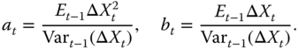
In the one period model

We want to find ![]() and
and ![]() minimizing
minimizing
This is the population version of a linear least-squares regression with the explanatory variable ![]() and the response variable
and the response variable ![]() . We obtain the solutions2
. We obtain the solutions2

and
The hedging coefficient can be written as

because constant ![]() can be removed from the covariance and the variance, and the discounting factors of the nominator and denominator cancel each other. Note that for a call option
can be removed from the covariance and the variance, and the discounting factors of the nominator and denominator cancel each other. Note that for a call option ![]() and for a put option
and for a put option ![]() .3
.3
We see that the quadratic price
is obtained by subtracting a correction term from the expected value of the payoff of the option.
The value process is useful in the multiperiod model, but in the single period model we can use the wealth process as well. We can use the following equivalent formulation. The initial wealth is ![]() . This amount is invested in the bank account. The amount
. This amount is invested in the bank account. The amount ![]() is borrowed at the risk-free rate and this money is invested in stock, so that there are
is borrowed at the risk-free rate and this money is invested in stock, so that there are ![]() stocks in the portfolio. The value of the portfolio at time 1 is
stocks in the portfolio. The value of the portfolio at time 1 is
We want to find values of ![]() and
and ![]() that minimize
that minimize
16.1.2.2 Scatter Plots of Stock Price Differences and Option Payoffs
Figure 16.1 shows a scatter plot of points ![]() together with linear fits. We use the daily data of S&P 500 prices, described in Section 2.4.1.
together with linear fits. We use the daily data of S&P 500 prices, described in Section 2.4.1.
We take ![]() and
and ![]() , where
, where ![]() are the gross returns of S&P 500 over 10 trading days. Values
are the gross returns of S&P 500 over 10 trading days. Values ![]() are the payoffs of call options with strike price
are the payoffs of call options with strike price ![]() , and the expiration time 10 trading days. In panel (a)
, and the expiration time 10 trading days. In panel (a) ![]() , and in panel (b)
, and in panel (b) ![]() . The green lines show the least-squares linear fit
. The green lines show the least-squares linear fit ![]() , where
, where ![]() and
and

where we use the sample means, variances, and covariances. The red lines show the linear fit ![]() , where
, where ![]() is the Black–Scholes price, and
is the Black–Scholes price, and ![]() is the Black–Scholes delta. The volatility is estimated by the sample standard deviation. We see that when
is the Black–Scholes delta. The volatility is estimated by the sample standard deviation. We see that when ![]() , there is hardly any difference between the least-squares fit and the Black–Scholes fit. When
, there is hardly any difference between the least-squares fit and the Black–Scholes fit. When ![]() , then the least-squares hedging coefficient is higher than the Black–Scholes delta.
, then the least-squares hedging coefficient is higher than the Black–Scholes delta.

Figure 16.1 Linear approximations of call payoffs. We show scatter plots of  for (a)
  and (b)
  . The green curves show the least-squares fit and the red curves show the Black–Scholes fit.
16.1.2.3 Pricing in the One Period Model Continued
We derive the solution (16.10), (16.11) in a different way. The different way of deriving the solution is such that it can be generalized to multiperiod models. Furthermore, it helps us to find the equivalent martingale measure and the hedging error.
We need to find ![]() and
and ![]() minimizing
minimizing
where ![]() and
and ![]() . We can write
. We can write
For a fixed ![]() the minimizer over
the minimizer over ![]() is
is

We have that

where we denote

and

We see from (16.17) that the mean-squared error is minimized by choosing ![]() . Equation (16.16) implies that the optimal hedging coefficient is
. Equation (16.16) implies that the optimal hedging coefficient is

where ![]() is defined in (16.18). The formulas (16.18) and (16.19) are equivalent with the formulas (16.10) and (16.11).4
is defined in (16.18). The formulas (16.18) and (16.19) are equivalent with the formulas (16.10) and (16.11).4
Note that formulas (16.18) and (16.19) define ![]() in terms of
in terms of ![]() , whereas (16.10) and (16.11) define
, whereas (16.10) and (16.11) define ![]() in terms of
in terms of ![]() .
.
16.1.2.4 The Martingale Measure in the One Period Model
Let us assume that our one period model is arbitrage-free. Theorem 13.1 implies that there exists an equivalent martingale measure. Theorem 13.2 implies that any arbitrage-free price can be written as an expected value ![]() for some equivalent martingale measure
for some equivalent martingale measure ![]() . Let us find the martingale measure
. Let us find the martingale measure ![]() , which is implied by the quadratic hedging.
, which is implied by the quadratic hedging.
The density of ![]() with respect to the underlying physical measure is obtained from (16.18) as
with respect to the underlying physical measure is obtained from (16.18) as

where

and

Now, we have found a measure ![]() such that
such that

Note that in our notation ![]() .
.
The Martingale Measure for S&P 500 in the One Period Model
Let us estimate the equivalent martingale measure associated with quadratic hedging using S&P 500 daily data of Section 2.4.1.
A time series of increments ![]() is not approximately stationary when the time series covers a long time period; see Figure 5.2. The time series of gross returns is nearly stationary, even when the time series extends over a long time period; see Figure 2.1(b). Thus, we can use historical simulation to create a time series of increments from the excess gross returns.
is not approximately stationary when the time series covers a long time period; see Figure 5.2. The time series of gross returns is nearly stationary, even when the time series extends over a long time period; see Figure 2.1(b). Thus, we can use historical simulation to create a time series of increments from the excess gross returns.
We take the interest rate ![]() . We consider a one-step model with the step of 20 days. The excess gross return is equal to the net return
. We consider a one-step model with the step of 20 days. The excess gross return is equal to the net return

Now,
Let
be the increment. Our S&P 500 data provides a sample of identically distributed observations ![]() from the distribution of
from the distribution of ![]() . We use non-overlapping increments.
. We use non-overlapping increments.
Let us estimate the density
of the martingale measure with respect to underlying physical measure of ![]() . The estimate is
. The estimate is
where ![]() and
and ![]() are estimates of
are estimates of ![]() and
and ![]() in (16.21), obtained by replacing the expectations and variances by sample averages and sample variances.
in (16.21), obtained by replacing the expectations and variances by sample averages and sample variances.
The underlying physical density of ![]() with respect to the Lebesgue measure can be estimated using the kernel estimate
with respect to the Lebesgue measure can be estimated using the kernel estimate ![]() of (3.43). The density of the martingale measure with respect to the Lebesgue measure can be estimated as
of (3.43). The density of the martingale measure with respect to the Lebesgue measure can be estimated as
Figure 16.2(a) shows the estimate ![]() of the density of the martingale measure with respect to the physical measure (dark green). The red curve shows the case of the Esscher measure and the blue curve the case of the Black–Scholes measure. The blue curve shows the density of the risk-neutral log-normal density with respect to the estimated physical measure. These are taken from Figure 13.1. Panel (b) shows the density
of the density of the martingale measure with respect to the physical measure (dark green). The red curve shows the case of the Esscher measure and the blue curve the case of the Black–Scholes measure. The blue curve shows the density of the risk-neutral log-normal density with respect to the estimated physical measure. These are taken from Figure 13.1. Panel (b) shows the density ![]() (dashed dark green) and
(dashed dark green) and ![]() (solid dark green). We show also the physical density (solid blue) and the risk-neutral density (dashed blue) in the Black–Scholes model.
(solid dark green). We show also the physical density (solid blue) and the risk-neutral density (dashed blue) in the Black–Scholes model.

Figure 16.2 Martingale measure in the one period model. (a) The density of the quadratic martingale measure with respect to the physical measure (dark green), Esscher measure (red), and Black–Scholes measure (blue). (b) The kernel density estimate of the physical measure (solid dark green), and the corresponding quadratic martingale measure (dashed dark green). The log-normal physical measure and the corresponding risk-neutral log-normal density are depicted as solid blue and dashed blue curves, respectively.
The Martingale Measure in the One Period Binomial Model
Let us study the one period binomial model, as defined in Section 14.2.1. In this model at time 0 the stock has value ![]() , and at time 1 the stock can take values
, and at time 1 the stock can take values ![]() and
and ![]() , where
, where ![]() . The probability of the up movement is
. The probability of the up movement is ![]() and the probability of the down movement is
and the probability of the down movement is ![]() with
with ![]() . Let us denote
. Let us denote
We have that
From (16.20) we obtain that the martingale measure ![]() satisfies
satisfies
where ![]() ,
, ![]() , and
, and ![]() or
or ![]() . We have that
. We have that
and
Thus,

which is equal to the martingale measure already derived in (14.18). In fact, the binomial model is a complete model and there is only one equivalent martingale measure.
16.1.3 The Two Period Model
We consider pricing and hedging of an European option in the two period model. The general multiperiod model is considered in Section 16.1.4, and this presentation includes the two period model as a special case. However, we think that it is easier to read the presentation of the multiperiod model when the two period model is presented first.
In the two period model the underlying security takes values ![]() ,
, ![]() , and
, and ![]() . The price
. The price ![]() is a fixed number and
is a fixed number and ![]() and
and ![]() are random variables. The option is written at time 0, and it expires at time 2. Hedging is done at times 0 and 1 by choosing the hedging coefficients
are random variables. The option is written at time 0, and it expires at time 2. Hedging is done at times 0 and 1 by choosing the hedging coefficients ![]() and
and ![]() . The value of the European option at the expiration is denoted by
. The value of the European option at the expiration is denoted by ![]() . For example, in the case of a call option
. For example, in the case of a call option ![]() , where
, where ![]() is the strike price.
is the strike price.
16.1.3.1 An Introduction to the Minimization Problem
The minimization problem can be solved either using the value process or by using the wealth process. The use of the value process is more convenient.
The Minimization Using the Value Process
In the two period model the value process and the discounted contingent claim are defined as

where ![]() ,
, ![]() ,
, ![]() , and
, and ![]() . We want to find
. We want to find ![]() minimizing
minimizing
Notation ![]() means the unconditional expectation with respect to the underlying measure
means the unconditional expectation with respect to the underlying measure ![]() , and we denote by
, and we denote by ![]() , the conditional expectation, with respect to sigma-algebra
, the conditional expectation, with respect to sigma-algebra ![]() :
:
Unlike in the one period model this minimization problem cannot be considered as a usual population version of a linear least squares regression. We can consider ![]() and
and ![]() as explanatory variables and
as explanatory variables and ![]() as the response variables, but now intercept
as the response variables, but now intercept ![]() and coefficient
and coefficient ![]() are chosen at time 0, and coefficient
are chosen at time 0, and coefficient ![]() is chosen at time 1. In the usual regression problem all parameters are chosen at time 0.
is chosen at time 1. In the usual regression problem all parameters are chosen at time 0.
The minimization problem can be solved in the following way. First, we find ![]() minimizing
minimizing
Let the minimizer be ![]() . The notation indicates that the minimizer depends on
. The notation indicates that the minimizer depends on ![]() and
and ![]() . Second, we find
. Second, we find ![]() and
and ![]() minimizing
minimizing
The Minimization Using the Wealth Process
The wealths at times 0, 1, and 2 are

where ![]() ,
, ![]() ,
, ![]() ,
, ![]() ,
, ![]() , and
, and ![]() . We want to find
. We want to find ![]() so that
so that
is minimized, under the self-financing constraints. The minimization problem can be solved in the following way. First, we find ![]() minimizing
minimizing
under the self-financing constraint
Let the minimizer be ![]() . The notation indicates that the minimizer depends on
. The notation indicates that the minimizer depends on ![]() . Second, we find
. Second, we find ![]() minimizing
minimizing
We can now see why it is easier to solve the problem using the value process: It is possible to apply unconstrained minimization when the value process is used.
16.1.3.2 Solving the Minimization Problem
Let us solve the problem of minimizing (16.22). We have that
Since
the minimizer over ![]() is
is

We have that

where we denote


and

It holds that
Similar calculations which lead to (16.23) show that the minimizer over ![]() is
is

Finally, we have to find ![]() minimizing
minimizing
The minimizer over ![]() is
is
where

Indeed, similar calculations which lead to (16.24) show that
where

We can summarize the results in the following proposition.
Note that hedging at time 1 is not done by coefficient ![]() in (16.23). Instead, at time 1 we consider the one period model between times 1 and 2, and choose the hedging coefficient of the one period model, as in (16.16).
in (16.23). Instead, at time 1 we consider the one period model between times 1 and 2, and choose the hedging coefficient of the one period model, as in (16.16).
16.1.3.3 The Martingale Measure in the Two Period Model
Let us find the martingale measure ![]() , which is implied by the quadratic hedging. We have to find such measure
, which is implied by the quadratic hedging. We have to find such measure ![]() that the option price is the discounted expectation with respect to the measure
that the option price is the discounted expectation with respect to the measure ![]() :
:
We obtain from (16.25) and (16.27) that the density of ![]() with respect to the underlying physical measure
with respect to the underlying physical measure ![]() is
is
where

In fact,
which can be written as

where we use the notation ![]() .
.
When the increments are independent, then the martingale measure ![]() is defined by the density
is defined by the density
where
and

compare this to ![]() and
and ![]() as defined in (16.21).
as defined in (16.21).
A Martingale Measure for S&P 500 in the Two Period Model
Let us estimate the equivalent martingale measure associated with quadratic hedging using S&P 500 daily data of Section 2.4.1. Let us consider a two-step model with two steps of 10 days. We take interest rate ![]() . Let
. Let
be the increments. Our S&P 500 data provides a sample of identically distributed observations from the distribution of ![]() . We use non-overlapping increments.
. We use non-overlapping increments.
Let us estimate the density
of martingale measure ![]() with respect to the physical measure
with respect to the physical measure ![]() .
.
First, we have to estimate ![]() and
and ![]() using nonparametric regression. Let us denote
using nonparametric regression. Let us denote
Let ![]() and
and ![]() be the kernel regression estimates.5
Then, we obtain the estimate of
be the kernel regression estimates.5
Then, we obtain the estimate of ![]() as
as

The estimate of ![]() is
is

Second, we have to estimate ![]() ,
, ![]() , and
, and ![]() . The estimates
. The estimates ![]() ,
, ![]() , and
, and ![]() are the sample averages. Then, we obtain the estimate of
are the sample averages. Then, we obtain the estimate of ![]() as
as

The estimate of ![]() is
is

Now, we have obtained the estimate
The density of the martingale measure with respect to the Lebesgue measure can be estimated as
where ![]() is a two-dimensional kernel density estimate of the underlying physical measure of
is a two-dimensional kernel density estimate of the underlying physical measure of ![]() . The kernel density estimator is defined in (3.43).
. The kernel density estimator is defined in (3.43).
When the returns are assumed to be independent, then we use the estimate
where
and ![]() and
and ![]() are the sample versions of
are the sample versions of

In the sample versions we replace the means and variances with the sample means and sample variances.
Figure 16.3 shows estimates of the density of the quadratic martingale measure with respect to the physical measure. In panel (a) we show estimate (16.28), which does not assume independence, and in panel (b) we show estimate (16.29), which assumes independence. In our setting regression estimation is difficult, and assuming independence leads to a more stable result. It is clear that the regression estimation could be improved by applying separate methods for the prediction of the first moment ![]() and for the second moment
and for the second moment ![]() .
.

Figure 16.3 The quadratic martingale measure: Two period model. Estimates of the density of the quadratic martingale measure with respect to the physical measure. (a) Increments are not assumed independent. (b) Increments are assumed to be independent.
16.1.4 The Multiperiod Model
We have derived the optimal hedging coefficient and the fair price in the mean-squared error sense for the two period model in Section 16.1.3. It is straightforward to generalize the results from the two period model to a general multiperiod model. The hedging coefficients and the fair price are derived using dynamic programming (backward induction).
16.1.4.1 Pricing in the Multiperiod Model
Let ![]() be the value process of a self-financing portfolio:
be the value process of a self-financing portfolio:

where
and ![]() . We want to find
. We want to find ![]() minimizing
minimizing
where ![]() is the discounted value of the derivative at the expiration.6
is the discounted value of the derivative at the expiration.6
When ![]() minimize (16.31), then we say that
minimize (16.31), then we say that ![]() is the fair price in the mean-squared error sense and
is the fair price in the mean-squared error sense and ![]() is the optimal hedging coefficient in the mean squared error sense. The coefficients
is the optimal hedging coefficient in the mean squared error sense. The coefficients ![]() are needed to derive
are needed to derive ![]() in our backward induction, but they do not equal the optimal hedging coefficients at times
in our backward induction, but they do not equal the optimal hedging coefficients at times ![]() . Instead, at time
. Instead, at time ![]() we need to make a new calculation of coefficients, say
we need to make a new calculation of coefficients, say ![]() , where
, where ![]() is the optimal hedging coefficient at time
is the optimal hedging coefficient at time ![]() .
.
The following theorem is proved in Černý (2004b, Section 13.4), where ![]() , so that the number of risky assets is allowed to be larger than one. Černý (2004a) is an article with the same result, and Bertsimas et al. (2001) contains a similar kind of result. A similar kind of proof can be found in Schäl (1994), who considers the case of mean self-financing strategies. The case of independent increments was considered by Wolczyńska (1998) and Hammarlid (1998).
, so that the number of risky assets is allowed to be larger than one. Černý (2004a) is an article with the same result, and Bertsimas et al. (2001) contains a similar kind of result. A similar kind of proof can be found in Schäl (1994), who considers the case of mean self-financing strategies. The case of independent increments was considered by Wolczyńska (1998) and Hammarlid (1998).
The Minimal Hedging Error
The proof implies that the minimal hedging error is given by ![]() , defined recursively in (16.36). Indeed, from (16.35) and (16.37), we obtain that
, defined recursively in (16.36). Indeed, from (16.35) and (16.37), we obtain that
The Hedging Coefficients
The proof implies that the sequence of quadratic hedging coefficients is given by

where ![]() . The coefficient
. The coefficient ![]() is applied at time 0, and the coefficients
is applied at time 0, and the coefficients ![]() will not be applied, because at time
will not be applied, because at time ![]() , we need to construct a model of
, we need to construct a model of ![]() periods.
periods.
Excess Gross Returns and Quadratic Hedging
The formulas for the price and the hedging coefficient are written using the increment
We can write the formulas as well using the excess gross return

The formulas (16.32) and (16.34) can be written as

where ![]() and
and

The fair price in the mean-squared error sense is ![]() and the optimal hedging coefficient at time
and the optimal hedging coefficient at time ![]() is
is

Indeed, we can multiply by ![]() and divide by
and divide by ![]() both the nominators and the denominators, and these terms can be moved inside the conditional expectations
both the nominators and the denominators, and these terms can be moved inside the conditional expectations ![]() , because they are
, because they are ![]() -measurable.
-measurable.
16.1.4.2 The Martingale Measure
Let us assume that the model is arbitrage-free. Theorem 13.1 says that there exists an equivalent martingale measure. Let us find the martingale measure ![]() associated with quadratic hedging. According to Theorem 13.2 the martingale measure is such that the option price is the discounted expectation with respect to the measure:
associated with quadratic hedging. According to Theorem 13.2 the martingale measure is such that the option price is the discounted expectation with respect to the measure:
The density of ![]() with respect to the underlying physical measure is
with respect to the underlying physical measure is

where

In fact, (16.32) in Theorem 16.2 implies that

which can be written as

where we use the notation ![]() . We can derive a similar expression for the density using the excess gross returns
. We can derive a similar expression for the density using the excess gross returns ![]() instead of increments
instead of increments ![]() : we can apply (16.38).
: we can apply (16.38).
16.1.4.3 Simplifying Assumptions
We can simplify the price formula (16.32) and the hedging formula (16.34) making restrictive assumptions on the increments ![]() . These assumptions are the martingale assumption, the assumption of a deterministic mean–variance ratio, the assumption of independence, and the assumption of independence and identical distribution.
. These assumptions are the martingale assumption, the assumption of a deterministic mean–variance ratio, the assumption of independence, and the assumption of independence and identical distribution.
Similar simplifications can be made to the formulas (16.38) and (16.39) when the assumptions are made on the process ![]() of the gross returns.7
of the gross returns.7
Quadratic Hedging Under the Martingale Assumption
Let us assume that  is a martingale with respect to the underlying physical measure
 ![]() . Then,
. Then,
![]() -almost surely. Thus,
-almost surely. Thus,
Now, we have that ![]() , and
, and
This implies that the option price is the expected value:
The first hedging coefficient is

where ![]() , and
, and ![]() . The expression for
. The expression for ![]() is the same as in the one period model; see (16.19), (16.10), and (16.12). Using the rule of iterated expectations we can also write
is the same as in the one period model; see (16.19), (16.10), and (16.12). Using the rule of iterated expectations we can also write

We can derive the result easily without using Theorem 16.2. Indeed,
where ![]() . Under the martingale assumption,
. Under the martingale assumption,

Also,

Thus, we obtain a sum of similar one period optimizations as in (16.15).
Deterministic Mean–Variance Ratio
Let us denote
Let us assume that the ratio
is deterministic for ![]() . This assumption is made in Föllmer and Schied (2002, Proposition 10.40, p. 396) to derive an expression for the variance-optimal hedging strategy. Note that the mean–variance ratio was used in (16.7) to formulate a sufficient condition for the existence and uniqueness of the variance-optimal hedging strategy (the bounded mean–variance trade-off). Under the assumption of a deterministic mean–variance ratio it holds that
. This assumption is made in Föllmer and Schied (2002, Proposition 10.40, p. 396) to derive an expression for the variance-optimal hedging strategy. Note that the mean–variance ratio was used in (16.7) to formulate a sufficient condition for the existence and uniqueness of the variance-optimal hedging strategy (the bounded mean–variance trade-off). Under the assumption of a deterministic mean–variance ratio it holds that ![]() in (16.33) is deterministic. In fact, now
in (16.33) is deterministic. In fact, now ![]() , and
, and

That is,

Values ![]() are defined recursively for
are defined recursively for ![]() by
by

where we start at ![]() . The fair price in the mean-squared error sense is
. The fair price in the mean-squared error sense is ![]() and the optimal hedging coefficient is
and the optimal hedging coefficient is

Independent Increments
Let us assume that the increments of discounted prices
are independent. Assume that the sigma-algebras are generated by the price process: ![]() . Then, the independence of increments implies that the conditional expectations reduce to unconditional expectations, and
. Then, the independence of increments implies that the conditional expectations reduce to unconditional expectations, and
are deterministic. Thus, the ratio ![]() is deterministic, and we obtain the price and hedging formulas (16.40) and (16.41).
is deterministic, and we obtain the price and hedging formulas (16.40) and (16.41).
i.i.d. Increments
Let us assume that the increments of discounted prices ![]() are independent and identically distributed. Let us denote
are independent and identically distributed. Let us denote
We have that

The price and hedging formulas are obtained from (16.40) and (16.41). Values ![]() are defined recursively for
are defined recursively for ![]() by
by

where we start at ![]() . The fair price in the mean-squared error sense is
. The fair price in the mean-squared error sense is ![]() and the optimal hedging coefficient is
and the optimal hedging coefficient is

The density of the martingale measure ![]() with respect to the underlying physical measure is
with respect to the underlying physical measure is

where

16.2 Local Quadratic Hedging
Local quadratic hedging applies a much simpler recursive scheme for minimizing the quadratic hedging error than global quadratic hedging of Section 16.1. Local quadratic hedging solves the minimization only approximately. This numerical error could be compensated if a more accurate statistical estimation is possible.
Local quadratic hedging reduces the minimization of quadratic hedging error to a series of minimizations in one period models. Thus, in the one period model global and local quadratic hedging are identical. We introduce local quadratic hedging using the two period model, and after that cover the multiperiod model.
16.2.1 The Two Period Model
We introduce local quadratic hedging using the two period model. In the two period model the value process and the discounted contingent claim are defined as

where ![]() ,
, ![]() ,
, ![]() , and
, and ![]() .
.
In local quadratic hedging the minimization is done in two steps.
- 1. First, we find
 and
and  minimizing

This is the population version of a linear least-squares regression with the response variable
 and the explanatory variable
  . The minimizers are
- 2. Second, we find
 and
and  minimizing

This is the population version of a linear least-squares regression with the response variable
 and the explanatory variable
  . The minimizers are
The minimization problems are easier to solve than in the case of global quadratic hedging. However, we are not able to minimize
but only to minimize it approximately.
We can write the price of the discounted contingent claim obtained by local quadratic hedging as
The first hedging coefficient ![]() can be written as
can be written as

The hedging coefficients ![]() and
and ![]() give the number of stocks in the hedging portfolio. The number of bonds
give the number of stocks in the hedging portfolio. The number of bonds ![]() and
and ![]() are obtained from the self-financing restrictions as in (16.3):
are obtained from the self-financing restrictions as in (16.3):

16.2.1.1 A Comparison to the Global Quadratic Hedging
To highlight the difference between the local and the global quadratic hedging, let us recall the global quadratic hedging of Section 16.1. In the global quadratic hedging we want to find ![]() minimizing
minimizing
The minimization problem can be solved in two steps. First, we find ![]() minimizing
minimizing
Let the minimizer be ![]() . The minimizer depends on
. The minimizer depends on ![]() and
and ![]() . Second, we find
. Second, we find ![]() and
and ![]() minimizing
minimizing
The quadratic price is ![]() .
.
16.2.1.2 The Martingale Measure
Let us study the martingale measure ![]() implied by the local hedging. The density of the martingale measure with respect to the physical measure
implied by the local hedging. The density of the martingale measure with respect to the physical measure ![]() is
is
where
with

for ![]() . The derivation of the martingale measure is given in (16.55) for the multiperiod model.
. The derivation of the martingale measure is given in (16.55) for the multiperiod model.
We can write the density in terms of the excess gross return. Namely,
where

and

for ![]() . This is possible, because the denominator and nominator can be multiplied by the square of
. This is possible, because the denominator and nominator can be multiplied by the square of ![]() , which is
, which is ![]() -measurable, and can be placed inside
-measurable, and can be placed inside ![]() .
.
A Martingale Measure for S&P 500: Two Steps
Let us estimate the equivalent martingale measure associated with quadratic hedging using S&P 500 daily data of Section 2.4.1. Let us consider a two-step model with two steps of 10 days. We choose interest rate ![]() . Let
. Let
be the price increments, where ![]() is the current time. When
is the current time. When ![]() runs through a long time period the observations are not stationary, but we can use our S&P 500 data to provide a sample of identically distributed observations of
runs through a long time period the observations are not stationary, but we can use our S&P 500 data to provide a sample of identically distributed observations of ![]() . We use non-overlapping increments. The observations are
. We use non-overlapping increments. The observations are

Let us estimate the density
of martingale measure ![]() with respect to the physical measure
with respect to the physical measure ![]() .
.
First, we have to estimate ![]() and
and ![]() using nonparametric regression. Let us denote
using nonparametric regression. Let us denote
Let ![]() and
and ![]() be the kernel regression estimates.8 Then, we obtain the estimates of
be the kernel regression estimates.8 Then, we obtain the estimates of ![]() and
and ![]() as
as

The estimate of ![]() is
is
Second, we have to estimate ![]() and
and ![]() . The estimates
. The estimates ![]() and
and ![]() are the sample averages. Then, we obtain the estimates of
are the sample averages. Then, we obtain the estimates of ![]() and
and ![]() as
as

The estimate of ![]() is
is
Now, we have obtained the estimate
The density of the martingale measure with respect to the Lebesgue measure can be estimated as
where ![]() is a two-dimensional kernel density estimate of the underlying physical measure of
is a two-dimensional kernel density estimate of the underlying physical measure of ![]() . The kernel density estimator is defined in (3.43).
. The kernel density estimator is defined in (3.43).
Figure 16.4 shows estimates of the density of the local quadratic martingale measure with respect to the physical measure. Panel (a) shows a contour plot and panel (b) shows a perspective plot.

Figure 16.4 A local quadratic martingale measure: Two period model. (a) A contour plot; (b) a perspective plot. Estimates of the density of the local quadratic martingale measure with respect to the physical measure.
16.2.2 The Multiperiod Model
Let
be the discounted value of the derivative at the expiration. We define recursively values ![]() and
and ![]() ,
, ![]() , starting with the value
, starting with the value ![]() . Let
. Let ![]() and
and ![]() be the minimizers of
be the minimizers of
for ![]() , over
, over ![]() , where
, where

This is a conditional population least-squares linear regression problem with the response variable ![]() and the explanatory variable
and the explanatory variable ![]() . The problem is similar to the minimization problem in the one period model of Section 16.1.2, but now we are conditioning on
. The problem is similar to the minimization problem in the one period model of Section 16.1.2, but now we are conditioning on ![]() . The solutions are
. The solutions are

and
Value ![]() is the price suggested by local quadratic hedging and
is the price suggested by local quadratic hedging and ![]() is the hedging coefficient at time 0, which is suggested by local quadratic hedging.
is the hedging coefficient at time 0, which is suggested by local quadratic hedging.
We can write ![]() using the undiscounted prices
using the undiscounted prices ![]() and
and ![]() as
as

where
The price can be written as:9

The hedging coefficients can be written as10

When ![]() are independent, then
are independent, then

where ![]() , and the price is
, and the price is

Also, similarly as in (14.34), when ![]() are independent,
are independent,

where ![]() .
.
16.2.2.1 A Comparison to Black–Scholes
We compare the quadratic prices and hedging coefficients to the Black–Scholes prices and hedging coefficients. We assume the independence of increments and use formulas (16.49) and (16.50). We apply S&P 500 daily data of Section 2.4.1. The Black–Scholes prices and deltas are computed using the annualized standard deviation as the volatility.
Figure 16.5 compares quadratically optimal prices to Black–Scholes prices. Panel (a) shows the quadratically optimal prices (black) and the Black–Scholes prices (red) as a function of moneyness ![]() . Time to expiration is 20 trading days. Panel (b) shows the ratios of the quadratically optimal prices to the Black–Scholes prices as a function of moneyness. Time to expiration is 20 days (black), 40 days (red), 60 days (blue), and 80 days (green). We see from panel (b) that when the moneyness is less than one, then the quadratic prices are less than the Black–Scholes prices. When the moneyness is about 0.95, then increasing the time to expiration makes the ratio of the quadratic prices to the Black–Scholes prices increase.
. Time to expiration is 20 trading days. Panel (b) shows the ratios of the quadratically optimal prices to the Black–Scholes prices as a function of moneyness. Time to expiration is 20 days (black), 40 days (red), 60 days (blue), and 80 days (green). We see from panel (b) that when the moneyness is less than one, then the quadratic prices are less than the Black–Scholes prices. When the moneyness is about 0.95, then increasing the time to expiration makes the ratio of the quadratic prices to the Black–Scholes prices increase.

Figure 16.5 Call prices. (a) The quadratic prices (black) and the Black–Scholes prices (red) as a function of moneyness  . (b) The ratios of the quadratic prices to the Black–Scholes prices. Time to expiration is 20 days (black), 40 days (red), 60 days (blue), and 80 days (green).
Figure 16.6 compares quadratic hedging coefficients to Black–Scholes hedging coefficients. Panel (a) shows the quadratic hedging coefficients (black) and the Black–Scholes hedging coefficients (red) as a function of moneyness ![]() . Time to expiration is 20 trading days. Panel (b) shows the ratios of the quadratic hedging coefficients to the Black–Scholes hedging coefficients as a function of moneyness. Time to expiration is 20 days (black), 40 days (red), 60 days (blue), and 80 days (green). We see from panel (b) that when the moneyness is about one, then increasing the time to expiration makes the ratio of the quadratic hedging coefficient to the Black–Scholes hedging coefficient increase. When the moneyness is less than 0.95 and the time to expiration is 20 days, then the quadratic hedging coefficient is much larger than the Black–Scholes hedging coefficient.
. Time to expiration is 20 trading days. Panel (b) shows the ratios of the quadratic hedging coefficients to the Black–Scholes hedging coefficients as a function of moneyness. Time to expiration is 20 days (black), 40 days (red), 60 days (blue), and 80 days (green). We see from panel (b) that when the moneyness is about one, then increasing the time to expiration makes the ratio of the quadratic hedging coefficient to the Black–Scholes hedging coefficient increase. When the moneyness is less than 0.95 and the time to expiration is 20 days, then the quadratic hedging coefficient is much larger than the Black–Scholes hedging coefficient.

Figure 16.6 Hedging coefficients. (a) The quadratic hedging coefficients (black) and the Black–Scholes hedging coefficients (red) as a function of moneyness  . (b) The ratios of the quadratic hedging coefficients to the Black–Scholes hedging coefficients. Time to expiration is 20 days (black), 40 days (red), 60 days (blue), and 80 days (green).
16.2.2.2 Square Integrability
The local quadratic trading strategy needs to be square integrable, in the sense of assumption (16.6). The square integrability is studied in Föllmer and Schied (2002, Proposition 10.10, p. 377). In fact, in order to guarantee the satisfaction of (16.6), it is enough to assume
![]() -almost surely, for
-almost surely, for ![]() , for a constant
, for a constant ![]() . Condition (16.51) of the bounded mean–variance trade-off appeared already in (16.7), where it was stated to guarantee the existence of a global quadratic trading strategy. Denote
. Condition (16.51) of the bounded mean–variance trade-off appeared already in (16.7), where it was stated to guarantee the existence of a global quadratic trading strategy. Denote ![]() . Assumption (16.51) implies that
. Assumption (16.51) implies that ![]() Thus we have for the local quadratic hedging coefficients
Thus we have for the local quadratic hedging coefficients ![]() that
that

where we used for the first equality the law of the iterated expectations, and for the third inequality the Cauchy–Schwarz inequality. Thus, the square integrability of ![]() implies the square integrability of
implies the square integrability of ![]() , which implies the square integrability of
, which implies the square integrability of ![]() . The backward induction shows that the square integrability of
. The backward induction shows that the square integrability of ![]() implies the square integrability of
implies the square integrability of ![]() for
for ![]() , under assumption (16.51).
, under assumption (16.51).
16.2.2.3 The Equivalent Martingale Measure
Let us find the equivalent martingale measure ![]() implied by the local quadratic hedging. The density of the martingale measure with respect to the physical measure
implied by the local quadratic hedging. The density of the martingale measure with respect to the physical measure ![]() is
is

where
with
In order that density ![]() is positive we have to assume that
is positive we have to assume that
![]() -almost surely on
-almost surely on ![]() . Otherwise,
. Otherwise, ![]() would be a signed measure and not a probability measure.
would be a signed measure and not a probability measure.
A Derivation of the Equivalent Martingale Measure
Let us show that
This follows because we can write

Now, we have

which can be written as

where we use the notation ![]() . Note that (16.56) implies that
. Note that (16.56) implies that
Characterizations of the Equivalent Martingale Measure
Measure ![]() in (16.52) can be characterized as a minimal martingale measure. Föllmer and Schied (2002, Definition 10.21, p. 382) define a minimal martingale measure to be such measure
in (16.52) can be characterized as a minimal martingale measure. Föllmer and Schied (2002, Definition 10.21, p. 382) define a minimal martingale measure to be such measure ![]() which is equivalent to
which is equivalent to ![]() ,
, ![]() , and such that every square integrable
, and such that every square integrable ![]() -martingale
-martingale ![]() which is strongly orthogonal to
which is strongly orthogonal to ![]() is also a
is also a ![]() -martingale. The strong orthogonality of
-martingale. The strong orthogonality of ![]() and
and ![]() means that
means that
![]() -almost surely, for
-almost surely, for ![]() .
.
Föllmer and Schied (2002, Theorem 10.22, p. 383) states that if ![]() is a minimal martingale measure, then (16.57) holds. Föllmer and Schied (2002, Corollary 10.28, p. 388) states that there exists at most one minimal martingale measure.
is a minimal martingale measure, then (16.57) holds. Föllmer and Schied (2002, Corollary 10.28, p. 388) states that there exists at most one minimal martingale measure.
Föllmer and Schied (2002, Theorem 10.30, p. 390) proves the existence and the uniqueness of a minimal martingale measure, and gives formula (16.58) for the density of the minimal martingale measure. Let us assume the condition (16.54) of positivity and the condition (16.51) of the bounded mean–variance trade-off. Then there exists a unique minimal martingale measure ![]() with density
with density
where ![]() and
and

with ![]() and
and

where ![]() is defined in (16.53), and
is defined in (16.53), and ![]() is the martingale part of the Doob decomposition of
is the martingale part of the Doob decomposition of ![]() . The Doob decomposition of
. The Doob decomposition of ![]() is
is
where ![]() is a martingale and
is a martingale and ![]() is predictable. The Doob decomposition is defined as
is predictable. The Doob decomposition is defined as

where ![]() ,
, ![]() , and
, and ![]() ; see Föllmer and Schied (2002, Proposition 6.1, p. 277).
; see Föllmer and Schied (2002, Proposition 6.1, p. 277).
Now we can show that the measure in (16.52) is the same as the minimal martingale measure in (16.58). Indeed,
and

16.2.3 Local Quadratic Hedging without Self-Financing
It is of interest to note that when we define a local quadratic hedging without self-financing, then the price will be the same, the hedging coefficients of the stocks will be the same, and only the hedging coefficients of the bonds will be different. A local quadratic hedging without self-financing can be defined in a similar way as the local quadratic hedging with self-financing, but we replace the value process with the wealth process.
16.2.3.1 Backward Induction
Let us consider the two period model with ![]() . Let us describe local quadratic hedging when the wealth process is used. The wealth at times 0, 1, and 2 is equal to
. Let us describe local quadratic hedging when the wealth process is used. The wealth at times 0, 1, and 2 is equal to

The self-financing condition would state that ![]() and
and ![]() should be chosen so that
should be chosen so that
In local quadratic hedging without self-financing we first find ![]() and
and ![]() minimizing
minimizing
This is the population version of a linear least-squares regression with the response variable ![]() and the explanatory variable
and the explanatory variable ![]() . The minimizers are
. The minimizers are

Let us denote
Term ![]() is obtained by “discounting” term
is obtained by “discounting” term ![]() . Second, we find
. Second, we find ![]() and
and ![]() minimizing
minimizing
This is the population version of a linear least-squares regression with the response variable ![]() and the explanatory variable
and the explanatory variable ![]() . The minimizers are
. The minimizers are

The optimal price in the local quadratic sense is
Term ![]() is obtained by “discounting” term
is obtained by “discounting” term ![]() . The price can be written as
. The price can be written as
The price is equal to the price which is obtained with the self-financing condition, as can be seen from (16.42). The first hedging coefficient can be written as

The hedging coefficient is equal to the hedging coefficient in (16.43), which is obtained with the self-financing restriction.
16.2.3.2 A Comparison with the Case of Self-Financing
We have seen that the price ![]() and the hedging coefficients
and the hedging coefficients ![]() and
and ![]() are the same whether the self-financing restriction is imposed or not. What about the coefficients
are the same whether the self-financing restriction is imposed or not. What about the coefficients ![]() and
and ![]() ? The quantities of the bonds are given by
? The quantities of the bonds are given by

The quantities can be compared to the quantities when the self-financing condition holds, given in (16.44) as

We see that ![]() are equal, but
are equal, but ![]() are different.11
are different.11
16.2.3.3 Mean Self-Financing
We have obtained a hedging strategy that is not self-financing, but it is mean self-financing, as defined in (16.5). Indeed,

because ![]() and
and ![]() since
since ![]() is
is ![]() -measurable and
-measurable and ![]() is
is ![]() -measurable.
-measurable.
16.3 Implementations of Local Quadratic Hedging
We have derived formulas for the quadratic price and the quadratic hedging coefficient. The formulas are not in a closed form but their application requires numerical methods. In addition, the formulas depend on the knowledge of the unknown data generating mechanism, and we need to use statistical methods to estimate the data generating mechanism.
We implement only the local quadratic hedging, both for the case when the increments are assumed to be independent, and for the case when the increments are assumed to be dependent.
Section 16.3.1 describes the basic setting of historical simulation. Section 16.3.2 describes numerical and statistical methods for the case of independent increments. Section 16.3.3 considers the case of dependent increments. Section 16.3.4 compares the implementations of quadratic pricing and hedging to some benchmarks.
16.3.1 Historical Simulation
To implement quadratic hedging we use historical simulation. Analogously, Monte Carlo simulation could be applied. In Monte Carlo simulation a statistical model is imposed, and sequences of observations are generated from the model. In historical simulation only the previous observations are used.
A similar type of implementation has been described in Potters et al. (2001), where price functions ![]() and hedging functions
and hedging functions ![]() are estimated using an expansion with basis functions, whereas we use kernel estimation. Also, we implement a method where the price function and the hedging function depend on volatility, so that they have the form
are estimated using an expansion with basis functions, whereas we use kernel estimation. Also, we implement a method where the price function and the hedging function depend on volatility, so that they have the form ![]() and
and ![]() .
.
16.3.1.1 Generating Sequences of Observations
We denote the time series of observed historical daily prices by ![]() . The price
. The price ![]() is the current price. We construct
is the current price. We construct ![]() sequences of prices:
sequences of prices:
where
Each sequence consists of ![]() values, and the initial price in each sequence is
values, and the initial price in each sequence is ![]() .
.
We may choose to use less than ![]() sequences, to make computation faster. Note that
sequences, to make computation faster. Note that ![]() sequences are overlapping, so that the use of the all possible
sequences are overlapping, so that the use of the all possible ![]() sequences may not increase statistical accuracy much, as compared for using a lesser number of sequences. We may construct
sequences may not increase statistical accuracy much, as compared for using a lesser number of sequences. We may construct ![]() sequences of prices, and to get non-overlapping sequences we may choose
sequences of prices, and to get non-overlapping sequences we may choose ![]() , and choose index
, and choose index ![]() to take the values
to take the values ![]() , for
, for ![]() .
.
16.3.1.2 The State Variable
With sequence ![]() of prices there is an associated sequence
of prices there is an associated sequence ![]() of state variables. Each
of state variables. Each ![]() can be a vector. We have constructed sequences
can be a vector. We have constructed sequences ![]() , which all start at the current stock price
, which all start at the current stock price ![]() . The values of the state variables that correspond to sequence
. The values of the state variables that correspond to sequence ![]() are
are
To utilize the information in the state variables, we use only those sequences ![]() that are such that at time
that are such that at time ![]() the value of the vector
the value of the vector ![]() of state variables is close to the current value
of state variables is close to the current value ![]() of the state variables. Let
of the state variables. Let ![]() be the collection of those times:
be the collection of those times:
where ![]() is the radius of the window, and
is the radius of the window, and ![]() is the Euclidean distance.
is the Euclidean distance.
For example, we can choose the state variable to be the logarithm of the current prediction of volatility:
where ![]() is estimated using the observed prices
is estimated using the observed prices ![]() . For instance, we can apply the GARCH(
. For instance, we can apply the GARCH(![]() ) volatility estimate.12Then
) volatility estimate.12Then ![]() is defined as
is defined as
where ![]() is the radius of the window. This is similar to the nonparametric GARCH-pricing in Section 15.3.
is the radius of the window. This is similar to the nonparametric GARCH-pricing in Section 15.3.
16.3.1.3 Heuristic Discussion
We want to solve a series of linear regression problems
for ![]() , where
, where ![]() . These regression problems are conditional on
. These regression problems are conditional on ![]() and
and ![]() . The solutions are functions
. The solutions are functions ![]() and
and ![]() , where
, where ![]() is the discounted value of the stock and
is the discounted value of the stock and ![]() is the value of the state variable. The sample version of the regression problem is
is the value of the state variable. The sample version of the regression problem is
where ![]() , and
, and ![]() .
.
In analogy, consider first the standard linear regression model
Assume we observe ![]() ,
, ![]() , from this model. Then,
, from this model. Then,
and we can estimate the constants ![]() and
and ![]() . Our setting resembles the model
. Our setting resembles the model
where ![]() is an additional random variable, and
is an additional random variable, and ![]() and
and ![]() are functions. Assume that we observe
are functions. Assume that we observe ![]() ,
, ![]() , from this model. Then
, from this model. Then
In order to estimate values ![]() and
and ![]() for a fixed
for a fixed ![]() we cannot use the standard linear regression, because there are no observations from model
we cannot use the standard linear regression, because there are no observations from model ![]() . Instead, we can estimate the functions
. Instead, we can estimate the functions ![]() and
and ![]() by localizing into the neighborhood of
by localizing into the neighborhood of ![]() . Let
. Let ![]() . Now, we can use linear regression for the observations
. Now, we can use linear regression for the observations
Note that we need to estimate functions ![]() and
and ![]() only at the points
only at the points ![]() and
and ![]() ,
, ![]() .
.
We need to estimate functions ![]() and
and ![]() of two arguments (where
of two arguments (where ![]() may be a vector). This can be done in two ways.
may be a vector). This can be done in two ways.
- 1. We can localize with respect to both
 and
and  .
. - 2. We can estimate function
Now, it is possible to avoid localization with respect to
 , make the localization only with respect to
  , and have available more observations to make the estimation. This is possible for certain
  .
.
Estimation of (16.61) is done by changing model (16.60) to model
where

An estimate ![]() leads to estimate
leads to estimate
Now the localization with respect to ![]() is not necessary when
is not necessary when ![]() , since
, since ![]() . In this case we can ignore the current level of the trajectory of the stock price.
. In this case we can ignore the current level of the trajectory of the stock price.
16.3.2 Local Quadratic Hedging Under Independence
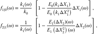
We apply the local quadratic hedging and assume independence of the increments. The hedging coefficients are given by the formula (16.49) as

where ![]() . The price is given by the formula (16.50) as
. The price is given by the formula (16.50) as

Here ![]() is the discounted payoff of the derivative,
is the discounted payoff of the derivative, ![]() , and
, and ![]() are the discounted prices of the risky asset.
are the discounted prices of the risky asset.
Let us assume for notational simplicity that the risk-free rate is zero, so that
The price ![]() involves only unconditional expectations, whereas hedging coefficients
involves only unconditional expectations, whereas hedging coefficients ![]() involve conditional expectations. In our implementation of the case of independent increments we make two simplifications, as compared to the previous heuristic discussion. First, the conditioning with respect to the state variable is done only at the time
involve conditional expectations. In our implementation of the case of independent increments we make two simplifications, as compared to the previous heuristic discussion. First, the conditioning with respect to the state variable is done only at the time ![]() of writing the option. Second, we do not need to move to the model (16.62), but we can handle the conditioning on the stock price
of writing the option. Second, we do not need to move to the model (16.62), but we can handle the conditioning on the stock price ![]() by renormalizing the tails of sequences
by renormalizing the tails of sequences ![]() so that they start with value
so that they start with value ![]() . This is possible because in the case of independent increments the intermediate values
. This is possible because in the case of independent increments the intermediate values ![]() for
for ![]() do not appear.
do not appear.
16.3.2.1 Unconditional Expectations
To estimate the unconditional expectations ![]() we apply sequences
we apply sequences ![]() in (16.59), where
in (16.59), where ![]() . These sequences give us the differences and the terminal values
. These sequences give us the differences and the terminal values
where ![]() . We estimate the unconditional expectations by
. We estimate the unconditional expectations by

16.3.2.2 Conditional Expectations
To estimate the hedging coefficients ![]() , when the stock price is
, when the stock price is ![]() , we renormalize the tails of the sequences. We define sequences such that the initial price is
, we renormalize the tails of the sequences. We define sequences such that the initial price is ![]() , and the number of observations in each sequence is
, and the number of observations in each sequence is ![]() , where
, where ![]() , that is, the length of the sequences is
, that is, the length of the sequences is ![]() . We define
. We define
where
![]() Now the initial price in each sequence is
Now the initial price in each sequence is ![]() .
.
We estimate the conditional expectations ![]() by applying sequences
by applying sequences ![]() in (16.63), where
in (16.63), where ![]() ,
, ![]() , and
, and ![]() . Each such sequence gives the differences and the terminal values
. Each such sequence gives the differences and the terminal values

The conditional expectations ![]() are estimated by
are estimated by

These estimates lead to the estimates of covariances and variances,13 and we obtain estimates of ![]() , which are used to produce an estimate of
, which are used to produce an estimate of ![]() .
.
16.3.2.3 Comparison to Black–Scholes
We compare prices and hedging coefficients of local quadratic hedging (with independence assumption) to the Black–Scholes prices and hedging coefficients.
Comparison to Black–Scholes Prices
Figure 16.7 shows the ratios of the locally quadratic prices (under independence) to the Black–Scholes prices as a function of the annualized volatility. In panel (a) moneyness is ![]() and in panel (b)
and in panel (b) ![]() . The smoothing parameter is
. The smoothing parameter is ![]() (black),
(black), ![]() (red), and
(red), and ![]() (blue). The time to expiration is 20 trading days.
(blue). The time to expiration is 20 trading days.

Figure 16.7 Call price ratios as a function of volatility. The ratios of the locally quadratic prices under independence to the Black–Scholes prices as a function of the annualized volatility. (a) Moneyness is  ; (b)
; (b)  . The smoothing parameter is
  (black),
  (red), and
  (blue).
Figure 16.8 shows the ratios of the locally quadratic prices to the Black–Scholes prices as a function of the moneyness ![]() . In panel (a) the time to expiration is
. In panel (a) the time to expiration is ![]() trading days, and in panel (b)
trading days, and in panel (b) ![]() . The annualized volatility is 0.1 (black), 0.2 (red), and 0.3 (blue). The smoothing parameter is
. The annualized volatility is 0.1 (black), 0.2 (red), and 0.3 (blue). The smoothing parameter is ![]() .
.

Figure 16.8 Call price ratios as a function of moneyness. The ratios of the locally quadratic prices under independence to the Black–Scholes prices as a function of moneyness  . (a)
. (a)  ; (b)
; (b)  . The annualized volatility is
  (black),
  (red), and
  (blue).
Figure 16.9 shows the ratios of the locally quadratic prices to the Black–Scholes prices as a function of the smoothing parameter ![]() . In panel (a) moneyness is
. In panel (a) moneyness is ![]() and in panel (b)
and in panel (b) ![]() . The annualized volatility is 0.1 (black), 0.2 (red), and 0.3 (blue). Time to expiration is
. The annualized volatility is 0.1 (black), 0.2 (red), and 0.3 (blue). Time to expiration is ![]() trading days.
trading days.

Figure 16.9 Call price ratios as a function of the smoothing parameter. The ratios of the locally quadratic prices under independence to the Black–Scholes prices as a function of smoothing parameter  . (a) Moneyness is
  ; (b)
; (b)  . The annualized volatility is
  (black),
  (red), and
  (blue).
Comparison to Black–Scholes Deltas
Figure 16.10 shows the ratios of the locally quadratic hedging coefficients (under independence) to the Black–Scholes deltas as a function of the annualized volatility. In panel (a) moneyness is ![]() and in panel (b)
and in panel (b) ![]() . The smoothing parameter is
. The smoothing parameter is ![]() (black),
(black), ![]() (red), and
(red), and ![]() (blue). The time to expiration is 20 trading days.
(blue). The time to expiration is 20 trading days.

Figure 16.10 Call hedging coefficient ratios as a function of volatility. The ratios of the locally quadratic hedging coefficients under independence to the Black–Scholes deltas as a function of the annualized volatility. (a) Moneyness is  ; (b)
; (b)  . The smoothing parameter is
  (black),
  (red), and
  (blue).
Figure 16.11 shows the ratios of the locally quadratic prices to the Black–Scholes prices as a function of the moneyness ![]() . In panel (a) time to expiration is
. In panel (a) time to expiration is ![]() trading days, and in panel (b)
trading days, and in panel (b) ![]() . The annualized volatility is 0.1 (black), 0.2 (red), and 0.3 (blue). The smoothing parameter is
. The annualized volatility is 0.1 (black), 0.2 (red), and 0.3 (blue). The smoothing parameter is ![]() .
.

Figure 16.11 Call hedging coefficient ratios as a function of moneyness. The ratios of the locally quadratic prices under independence to the Black–Scholes prices as a function of moneyness  . (a)
. (a)  ; (b)
; (b)  . The annualized volatility is
  (black),
  (red), and
  (blue).
Figure 16.12 shows the ratios of the locally quadratic hedging coefficients to the Black–Scholes deltas as a function of the smoothing parameter ![]() . In panel (a) moneyness is
. In panel (a) moneyness is ![]() and in panel (b)
and in panel (b) ![]() . The annualized volatility is 0.1 (black), 0.2 (red), and 0.3 (blue). Time to expiration is
. The annualized volatility is 0.1 (black), 0.2 (red), and 0.3 (blue). Time to expiration is ![]() trading days.
trading days.

Figure 16.12 Call hedging coefficient ratios as a function of smoothing parameter. The ratios of the locally quadratic hedging coefficients under independence to the Black–Scholes deltas as a function of smoothing parameter  . (a) Moneyness is
  ; (b)
; (b)  . The annualized volatility is
  (black),
  (red), and
  (blue).
16.3.3 Local Quadratic Hedging under Dependence
We apply local quadratic hedging without assuming independence of increments. We need to estimate the sequences

where ![]() . The recursion starts with the known value
. The recursion starts with the known value ![]() .
.
Let us assume for notational simplicity that the risk-free rate is zero, so that
Let us denote by ![]() the observed values of the stock
the observed values of the stock ![]() , and let us denote by
, and let us denote by ![]() the observed values of the state variable
the observed values of the state variable ![]() . The values in sequence
. The values in sequence ![]() , defined in (16.59), are denoted by
, defined in (16.59), are denoted by
where ![]() . The corresponding sequence of the values of the state variables is
. The corresponding sequence of the values of the state variables is
In the case of local quadratic hedging under independence the formulas did not involve the intermediate values ![]() for
for ![]() . This simplified the computations, and we needed only to renormalize the tails of the price trajectories. Now we use a technique where we move from the increments
. This simplified the computations, and we needed only to renormalize the tails of the price trajectories. Now we use a technique where we move from the increments ![]() to the net returns
to the net returns ![]() of stock prices, and from the values
of stock prices, and from the values ![]() to the values
to the values ![]() , where
, where
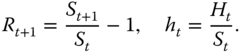
We can write

We need to estimate the conditional expectations
The conditional expectations are interpreted as
16.3.3.1 The Steps of Backward Induction
Consider step ![]() . Assume that we have produced estimates
. Assume that we have produced estimates
where
Step ![]() is the first step of the backward induction. When
is the first step of the backward induction. When ![]() , then in the case of a call option
, then in the case of a call option
where ![]() ,
, ![]() , are the terminal values of sequences
, are the terminal values of sequences ![]() .
.
We estimate the conditional expectations first with local averaging, and then generalize to kernel estimation.
Local Averaging
Let
Set ![]() contains those indexes
contains those indexes ![]() for which the
for which the ![]() th element
th element ![]() is close to
is close to ![]() , where
, where ![]() . Note that
. Note that ![]() . Let
. Let
We estimate for each ![]() the conditional expectations by14
the conditional expectations by14

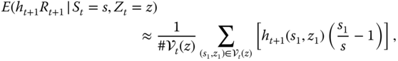
These estimates lead to the estimates of covariances and variances, and we obtain an estimate of ![]() . An estimate for
. An estimate for ![]() is obtained by
is obtained by
for ![]() and
and ![]() , where
, where ![]() . Note that at step
. Note that at step ![]() set
set ![]() is a singleton:
is a singleton:
The price is obtained as
and the first hedging coefficient is
Kernel Estimation
The estimation of the conditional expectations can be done by using kernel estimation. We estimate for each ![]() the conditional expectations using the estimators
the conditional expectations using the estimators
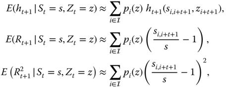

where the weights are defined as

![]() is the scaled kernel
is the scaled kernel ![]() ,
, ![]() is a kernel function, where
is a kernel function, where ![]() is the dimension of vector
is the dimension of vector ![]() . The previous method of local averaging is obtained as a special case when the kernel function is chosen as
. The previous method of local averaging is obtained as a special case when the kernel function is chosen as
These estimates lead to the estimates of covariances and variances, and we obtain an estimate of ![]() . An estimate of
. An estimate of ![]() is obtained using the formula (16.65).
is obtained using the formula (16.65).
16.3.3.2 Comparison to Black–Scholes
We compare both prices and hedging coefficients of local quadratic hedging to the Black–Scholes prices and hedging coefficients.
Comparison to Black–Scholes Prices
Figure 16.13 shows the ratios of the locally quadratic prices to the Black–Scholes prices as a function of the annualized volatility. In panel (a) moneyness is ![]() and in panel (b)
and in panel (b) ![]() . The smoothing parameter is
. The smoothing parameter is ![]() (black),
(black), ![]() (red), and
(red), and ![]() (blue). Time to expiration is 20 trading days.
(blue). Time to expiration is 20 trading days.

Figure 16.13 Call price ratios as a function of volatility under dependence. The ratios of the locally quadratic prices to the Black–Scholes prices as a function of the annualized volatility. (a) Moneyness is  ; (b)
; (b)  . The smoothing parameter is
  (black),
  (red), and
  (blue).
Figure 16.14 shows the ratios of the locally quadratic prices to the Black–Scholes prices as a function of the moneyness ![]() . In panel (a) time to expiration is
. In panel (a) time to expiration is ![]() trading days, and in panel (b)
trading days, and in panel (b) ![]() . The annualized volatility is 0.1 (black), 0.2 (red), and 0.3 (blue). The smoothing parameter is
. The annualized volatility is 0.1 (black), 0.2 (red), and 0.3 (blue). The smoothing parameter is ![]() .
.

Figure 16.14 Call price ratios as a function of moneyness: Dependence. The ratios of the locally quadratic prices under dependence to the Black–Scholes prices as a function of moneyness  . (a)
. (a)  ; (b)
; (b)  . The annualized volatility is
  (black),
  (red), and
  (blue).
Figure 16.15 shows the ratios of the locally quadratic prices to the Black–Scholes prices as a function of the smoothing parameter ![]() . In panel (a) moneyness is
. In panel (a) moneyness is ![]() and in panel (b)
and in panel (b) ![]() . The annualized volatility is 0.1 (black), 0.2 (red), and 0.3 (blue). Time to expiration is
. The annualized volatility is 0.1 (black), 0.2 (red), and 0.3 (blue). Time to expiration is ![]() trading days.
trading days.

Figure 16.15 Call price ratios as a function of the smoothing parameter: Dependence. The ratios of the locally quadratic prices under dependence to the Black–Scholes prices as a function of smoothing parameter  . (a) Moneyness is
  ; (b)
; (b)  . The annualized volatility is
  (black),
  (red), and
  (blue).
Comparison to Black–Scholes Deltas
Figure 16.16 shows the ratios of the locally quadratic hedging coefficients (under dependence) to the Black–Scholes deltas as a function of the annualized volatility. In panel (a) moneyness is ![]() and in panel (b)
and in panel (b) ![]() . The smoothing parameter is
. The smoothing parameter is ![]() (black),
(black), ![]() (red), and
(red), and ![]() (blue). Time to expiration is 20 trading days.
(blue). Time to expiration is 20 trading days.

Figure 16.16 Call hedging coefficient ratios as a function of volatility: Dependence. The ratios of the locally quadratic hedging coefficients under dependence to the Black–Scholes deltas as a function of the annualized volatility. (a) Moneyness is  ; (b)
; (b)  . The smoothing parameter is
  (black),
  (red), and
  (blue).
Figure 16.17 shows the ratios of the locally quadratic prices to the Black–Scholes prices as a function of the moneyness ![]() . In panel (a) time to expiration is
. In panel (a) time to expiration is ![]() trading days, and in panel (b)
trading days, and in panel (b) ![]() . The annualized volatility is 0.1 (black), 0.2 (red), and 0.3 (blue). The smoothing parameter is
. The annualized volatility is 0.1 (black), 0.2 (red), and 0.3 (blue). The smoothing parameter is ![]() .
.

Figure 16.17 Call hedging coefficient ratios as a function of moneyness: Dependence. The ratios of the locally quadratic prices under dependence to the Black–Scholes prices as a function of moneyness  . (a)
. (a)  ; (b)
; (b)  . The annualized volatility is
  (black),
  (red), and
  (blue).
Figure 16.18 shows the ratios of the locally quadratic hedging coefficients to the Black–Scholes deltas as a function of the smoothing parameter ![]() . In panel (a) moneyness is
. In panel (a) moneyness is ![]() and in panel (b)
and in panel (b) ![]() . The annualized volatility is 0.1 (black), 0.2 (red), and 0.3 (blue). Time to expiration is
. The annualized volatility is 0.1 (black), 0.2 (red), and 0.3 (blue). Time to expiration is ![]() trading days.
trading days.

Figure 16.18 Call hedging coefficient ratios as a function of smoothing parameter: Dependence. The ratios of the locally quadratic hedging coefficients under dependence to the Black–Scholes deltas as a function of smoothing parameter  . (a) Moneyness is
  ; (b)
; (b)  . The annualized volatility is
  (black),
  (red), and
  (blue).
16.3.4 Evaluation of Quadratic Hedging
Figure 16.19 shows (a) tail plots and (b) kernel density estimates of hedging errors for call options.15 The blue curves show the case of Black–Scholes hedging. The local quadratic hedging is done assuming independence and the smoothing parameter is ![]() (red),
(red), ![]() (dark green),
(dark green), ![]() (purple), and
(purple), and ![]() (orange). The volatility is in all cases the GARCH(
(orange). The volatility is in all cases the GARCH(![]() ) volatility. The moneyness of call options is
) volatility. The moneyness of call options is ![]() . Time to maturity is 20 days and hedging is done every day. Tail plots are defined in Section 3.2.1 and the kernel density estimator is defined in Section 3.2.2. We apply the standard normal kernel function and the smoothing parameter of the density estimator is chosen by the normal reference rule. We see from panel (b) that smoothing parameters
. Time to maturity is 20 days and hedging is done every day. Tail plots are defined in Section 3.2.1 and the kernel density estimator is defined in Section 3.2.2. We apply the standard normal kernel function and the smoothing parameter of the density estimator is chosen by the normal reference rule. We see from panel (b) that smoothing parameters ![]() lead to similar results, but smoothing parameter
lead to similar results, but smoothing parameter ![]() leads to a more dispersed distribution. Black–Scholes hedging leads to a more concentrated distribution than the quadratic hedging with independence assumption, but the quadratic hedging leads to a distribution which is skewed to the right in the central area of the distribution, which means that there are more gains than losses for the hedger of the option.
leads to a more dispersed distribution. Black–Scholes hedging leads to a more concentrated distribution than the quadratic hedging with independence assumption, but the quadratic hedging leads to a distribution which is skewed to the right in the central area of the distribution, which means that there are more gains than losses for the hedger of the option.

Figure 16.19 Distribution of hedging errors: Local quadratic with independence. Shown are (a) tail plots and (b) kernel density estimates of hedging errors. Black–Scholes hedging (blue), local quadratic hedging with independence using the smoothing parameter  (red),
  (dark green),
  (purple), and
  (orange).

Figure 16.20 Distribution of hedging errors when hedging is done once: Local quadratic under independence and dependence. Shown are (a) tail plots and (b) kernel density estimates of hedging errors. Black–Scholes hedging (blue), local quadratic hedging with independence (green), and local quadratic hedging with dependence (red).
Figure 16.20 considers the case of hedging only once. Panel (a) shows tail plots and panel (b) shows kernel density estimates of hedging errors. The moneyness of call options is ![]() . Time to maturity is 20 days. The blue curves show the case of Black–Scholes hedging. The red curves show the case of local quadratic hedging assuming dependence. The green curves show the case of local quadratic hedging assuming independence. The smoothing parameter is in both cases
. Time to maturity is 20 days. The blue curves show the case of Black–Scholes hedging. The red curves show the case of local quadratic hedging assuming dependence. The green curves show the case of local quadratic hedging assuming independence. The smoothing parameter is in both cases ![]() . The volatility is in all cases the GARCH(
. The volatility is in all cases the GARCH(![]() ) volatility.
) volatility.

Figure 16.21 Distribution of hedging errors with daily hedging: Local quadratic under independence and dependence. Shown are (a) tail plots and (b) kernel density estimates of hedging errors. Black–Scholes hedging (blue), local quadratic hedging with independence (green), and local quadratic hedging with dependence (red).
Figure 16.21 shows (a) tail plots and (b) kernel density estimates of hedging errors. The moneyness of call options is ![]() . Time to maturity is 20 days and hedging is done every day. The blue curves show the case of Black–Scholes hedging. The red curves show the case of local quadratic hedging assuming dependence. The green curves show the case of local quadratic hedging assuming independence. The smoothing parameter is in both cases
. Time to maturity is 20 days and hedging is done every day. The blue curves show the case of Black–Scholes hedging. The red curves show the case of local quadratic hedging assuming dependence. The green curves show the case of local quadratic hedging assuming independence. The smoothing parameter is in both cases ![]() . The volatility is in all cases the GARCH(
. The volatility is in all cases the GARCH(![]() ) volatility.
) volatility.

From the second equation we get

From the first equation we get ![]() . Inserting this to (16.9) gives
. Inserting this to (16.9) gives

It holds that


Inserting this to (16.19) gives
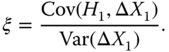

where ![]() ,
, ![]() , are the observations from the distribution of
, are the observations from the distribution of ![]() ,
,

![]() is a kernel function and
is a kernel function and ![]() is a smoothing parameter.
is a smoothing parameter.
where ![]() is the wealth, and
is the wealth, and ![]() is the value of the option at the expiration.
is the value of the option at the expiration.


where ![]() ,
, ![]() , are the observations of
, are the observations of ![]() ,
, ![]() is a kernel function and
is a kernel function and ![]() is a smoothing parameter.
is a smoothing parameter.

On the other hand, ![]()

and the generalization of (16.48) to ![]() :
:


Let us define the objective function
which is to be minimized with respect to ![]() ,
, ![]() ,
, ![]() , and
, and ![]() . However, this optimization problem is not easier to solve than the global quadratic optimization.
. However, this optimization problem is not easier to solve than the global quadratic optimization.
where ![]() ,
, ![]() . Prediction
. Prediction ![]() is made at time
is made at time ![]() , and it predicts the volatility at time
, and it predicts the volatility at time ![]() . In order to obtain initial estimates of parameters
. In order to obtain initial estimates of parameters ![]() ,
, ![]() ,
, ![]() , and an initial value
, and an initial value ![]() for the volatility, we assume that there are available observations
for the volatility, we assume that there are available observations ![]() . It is reasonable to update the estimates
. It is reasonable to update the estimates ![]() ,
, ![]() , and
, and ![]() sequentially, using data
sequentially, using data ![]() .
.