
Chapter 15
Pricing in Incomplete Models
We give an overview of various approaches to price derivatives in incomplete markets. In an incomplete market, there exists derivatives which cannot be exactly replicated. The second fundamental theorem of asset pricing (Theorem 13.3) states that if the market is arbitrage-free and complete, then there is only one equivalent martingale measure, and thus there is only one arbitrage-free price. When the arbitrage-free market is not complete, then there are many equivalent martingale measures, and thus there are many arbitrage-free prices.
In this chapter, we describe some approaches for choosing the equivalent martingale measure from a set of available equivalent martingale measures, in the case of an incomplete market. Chapter 16 is devoted to the study of quadratic hedging and pricing. In this chapter, we give only a short description of quadratic pricing, and concentrate to describe other methods.
Utility maximization provides a general method for the construction of an equivalent martingale measure. We show that the Esscher measure, which was used to prove the first fundamental theorem of asset pricing (Theorem 13.1), is related to the maximization of the expected utility, when the utility function is the exponential utility function. The concept of marginal rate of substitution provides a heuristic way to connect the utility maximization to the pricing of options. Minimizing the relative entropy between a martingale measure and the physical measure provides an equally natural way to construct an equivalent martingale measure. Again, we can show that minimizing the relative entropy is related to the maximizing the expected utility with the exponential utility function. It is of interest to compare the Esscher prices to the Black–Scholes prices: we see that the Esscher prices are close to the Black–Scholes prices for at-the-money calls, whereas for out-of-the-money calls the Esscher prices are lower.
We describe formulas for constructing an equivalent martingale measure by an absolutely continuous change of measure. These formulas are given for conditionally Gaussian returns, and for conditionally Gaussian logarithmic returns. An absolutely continuous change of measure shifts the market measure so that it becomes risk-neutral.
GARCH models provide good volatility predictions, and it is natural to ask whether GARCH models could be suitable for pricing options. We can apply the absolutely continuous change of measure to obtain an equivalent martingale measure in the GARCH market model. The standard GARCH(![]() ) model can be modified so that we obtain a model where the prices can be expressed almost in a closed form. We still need a numerical integration to compute the prices, but Monte Carlo simulation of price trajectories is not needed. The modified GARCH(
) model can be modified so that we obtain a model where the prices can be expressed almost in a closed form. We still need a numerical integration to compute the prices, but Monte Carlo simulation of price trajectories is not needed. The modified GARCH(![]() ) model was presented in Heston and Nandi (2000).
) model was presented in Heston and Nandi (2000).
It is on interest to construct a nonparametric pricing method, and compare its properties to other methods. We construct a method which combines historical simulation, the Esscher measure, and conditioning on the current volatility.
An equivalent martingale measure can be deduced from the market prices of the options. This martingale measure could be called the implied martingale measure, because there is an analogy to the implied volatility. When the implied martingale measure is used, we have to assume that the market prices of the options are rational. This requires that we use option prices of liquid markets to estimate the implied martingale measure. The implied martingale measure which is deduced from the prices of liquid options can be used to price illiquid options.
Section 15.1 describes quadratic hedging and pricing. Section 15.2 describes pricing with the help of utility maximization. Section 15.3 considers pricing with the help of absolutely continuous changes of measures (Girsanov's theorem). Section 15.4 describes the use of a GARCH model in option pricing. Section 15.5 describes a method of nonparametric pricing which uses historical simulation. Section 15.6 discusses pricing with the help of estimating the risk-neutral density. Section 15.7 mentions quantile hedging.
Pricing in incomplete markets is studied in Duffie and Skiadas (1994), El Karoui and Quenez (1995), Karatzas (1996), and Gourioux et al. (1998). Bingham and Kiesel (2004, Chapter 7) discuss pricing in incomplete models, including mean–variance hedging and models driven by Lévy processes. Pricing of derivatives in the context of general econometric theory is presented in Magill and Quinzii (1996). Further references include Karatzas and Kou (1996).
15.1 Quadratic Hedging and Pricing
Quadratic hedging and pricing is discussed in detail in Chapter 16 (see also Föllmer and Schied, 2002, Definition 10.36, p. 393). At this point, we give a brief summary of the method.
Let us explain the idea of quadratic hedging using the case with one risky asset (![]() ) and two periods (
) and two periods (![]() ). The initial wealth is
). The initial wealth is ![]() and the wealth obtained by trading with a bond and a stock is
and the wealth obtained by trading with a bond and a stock is
where ![]() is the price of the bond,
is the price of the bond, ![]() is the price of the stock,
is the price of the stock, ![]() is the number of bonds in the portfolio, and
is the number of bonds in the portfolio, and ![]() is the number of stocks in the portfolio. Our aim is to replicate the terminal value
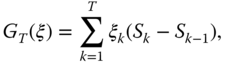
is the number of stocks in the portfolio. Our aim is to replicate the terminal value ![]() of the contingent claim. We measure the quality of the approximation by the quadratic hedging error
of the contingent claim. We measure the quality of the approximation by the quadratic hedging error
The minimization is done over self-financing trading strategies and over the initial wealth ![]() . The self-financing means that
. The self-financing means that ![]() and
and ![]() satisfy
satisfy
The self-financing restriction connects the initial wealth ![]() to the final wealth
to the final wealth ![]() . The quadratic price is the initial wealth
. The quadratic price is the initial wealth ![]() that minimizes the quadratic hedging error.
that minimizes the quadratic hedging error.
The minimization is done easier when we use the value process, instead of the wealth process. Our final formulation for the general case ![]() and
and ![]() will be the following. In quadratic hedging, the quadratic hedging error
will be the following. In quadratic hedging, the quadratic hedging error
is minimized among strategies ![]() 1 and among the initial investment
1 and among the initial investment ![]() , where
, where ![]() is the discounted contingent claim. The terminal value of the gains process is defined by
is the discounted contingent claim. The terminal value of the gains process is defined by

where ![]() is the discounted price vector.
is the discounted price vector.
15.2 Utility Maximization
It turns out that an equivalent martingale measure can be found by looking at the portfolios which maximize the expected utility. Section 15.2.1 shows that the Esscher martingale measure is related to the maximization of the expected utility with the exponential utility function. Section 15.2.2 considers other utility functions. Section 15.2.3 shows that the Esscher measure is the equivalent martingale measure which minimizes the relative entropy with respect to the physical measure. Section 15.2.4 computes examples of Esscher prices. Section 15.2.5 discusses the heuristics of the marginal rate of substitution.
The use of Esscher transform and more general methods of utility maximization has to be combined with the estimation of the underlying distribution of the stock price process. This issue has been addressed in Bühlmann et al. (1996), Siu et al. (2004), Christoffersen et al. (2006), and Chorro et al. (2012), where parametric modeling was used. We address the issue in Section 15.5, where a nonparametric estimation is applied (see also Section 15.2.4).
15.2.1 The Exponential Utility
The Esscher transformation was applied in the proof of Theorem 13.1 (the first fundamental theorem of asset pricing) to construct an equivalent martingale measure in an arbitrage-free market. Let us recall the definition of the Esscher measure for the case of one risky asset. Let ![]() be the discounted stock price, where
be the discounted stock price, where ![]() . Let
. Let
Let
where ![]() . Let
. Let
be the unique finite minimizer of ![]() over
over ![]() . Let
. Let ![]() and
and

for ![]() . We define the probability measure
. We define the probability measure
Now ![]() ,
, ![]() , and
, and ![]() for
for ![]() . Hence
. Hence ![]() is a martingale difference and
is a martingale difference and ![]() is a martingale with respect to
is a martingale with respect to ![]() .
.
The Esscher martingale measure is related to the maximization of the expected utility with the exponential utility function. The exponential utility function is defined as
where ![]() is the parameter of risk aversion. We want to maximize
is the parameter of risk aversion. We want to maximize
over self-financing trading strategies ![]() , where
, where

The maximization is equivalent to the minimization of
We can write

where ![]() . Minimization of
. Minimization of
over ![]() -measurable
-measurable ![]() is equivalent to the minimization of
is equivalent to the minimization of
over ![]() . Thus, we arrive at the minimizer
. Thus, we arrive at the minimizer ![]() in (15.1), and we can define an equivalent martingale measure (15.2) with the help of these minimizers.
in (15.1), and we can define an equivalent martingale measure (15.2) with the help of these minimizers.
15.2.2 Other Utility Functions
The construction of the Esscher martingale measure can be generalized to cover other utility functions. For example, consider the one period model with ![]() risky assets and let
risky assets and let ![]() be the vector of discounted net gains:
be the vector of discounted net gains:
where ![]() are the prices of the risky assets at time
are the prices of the risky assets at time ![]() . Föllmer and Schied (2002, Corollary 3.10) states that if the market is arbitrage-free, and the utility function
. Föllmer and Schied (2002, Corollary 3.10) states that if the market is arbitrage-free, and the utility function ![]() and a maximizer
and a maximizer ![]() of
of ![]() satisfy certain assumptions,2 then
satisfy certain assumptions,2 then

defines an equivalent martingale measure ![]() .
.
The proof is based on the fact that a martingale measure has to satisfy ![]() , and this follows for the measure defined in (15.3) because the maximizer satisfies the first-order condition
, and this follows for the measure defined in (15.3) because the maximizer satisfies the first-order condition ![]() . Note that the existence of a maximizer is implied by Föllmer and Schied (2002, Theorem 3.3).
. Note that the existence of a maximizer is implied by Föllmer and Schied (2002, Theorem 3.3).
The Esscher density
is a special case of (15.3). Indeed, when the utility function is the exponential utility function ![]() , where
, where ![]() and
and ![]() is the risk aversion, then (15.3) gives the density
is the risk aversion, then (15.3) gives the density
Portfolio ![]() maximizes the expected utility
maximizes the expected utility ![]() if and only if
if and only if ![]() minimizes the moment generating function
minimizes the moment generating function ![]() . Thus, we obtain the density in (15.4), and the martingale measure
. Thus, we obtain the density in (15.4), and the martingale measure ![]() is independent of the risk aversion
is independent of the risk aversion ![]() .
.
Note that we have maximized ![]() over
over ![]() , which is not the same as maximizing the expected utility of the wealth. However, in the one-period case the wealth is written in (9.9) as
, which is not the same as maximizing the expected utility of the wealth. However, in the one-period case the wealth is written in (9.9) as
Let ![]() be a strictly increasing, strictly concave, and continuous utility function. We want to find
be a strictly increasing, strictly concave, and continuous utility function. We want to find ![]() which maximizes
which maximizes ![]() over all
over all ![]() such that
such that ![]() is
is ![]() -almost surely in the domain of
-almost surely in the domain of ![]() . Define
. Define
The original utility maximization is equivalent to the maximization of
among all ![]() such that
such that ![]() , where
, where ![]() is the domain of
is the domain of ![]() .
.
15.2.3 Relative Entropy
The Esscher martingale measure was shown to be related to the maximization of the expected utility with the exponential utility function. We can also show that the Esscher measure can be obtained by minimizing the Kullback–Leibler distance to the physical market measure.
The closeness of probability distributions can be measured by the relative entropy (the Kullback–Leibler distance). The relative entropy of a probability measure ![]() with respect to a probability measure
with respect to a probability measure ![]() is defined as
is defined as

when ![]() dominates
dominates ![]() . When
. When ![]() does not dominate
does not dominate ![]() , then we define
, then we define ![]() .
.
Föllmer and Schied (2002, Corollary 3.25) states the following result for the one-period model with ![]() risky assets: When the market model is arbitrage-free, then there exists a unique equivalent martingale measure
risky assets: When the market model is arbitrage-free, then there exists a unique equivalent martingale measure ![]() , which minimizes the relative entropy
, which minimizes the relative entropy ![]() over all
over all ![]() , where
, where ![]() is the set of equivalent martingale measures. Furthermore, the density of
is the set of equivalent martingale measures. Furthermore, the density of ![]() is the Esscher density
is the Esscher density
where ![]() is the minimizer of the moment generating function
is the minimizer of the moment generating function ![]() , and
, and ![]() is the vector of discounted net gains:
is the vector of discounted net gains: ![]() , where
, where ![]() is the vector of prices at time
is the vector of prices at time ![]() , and
, and ![]() is the vector of prices at time
is the vector of prices at time ![]() .
.
15.2.4 Examples of Esscher Prices
We apply the data of S&P 500 daily prices, described in Section 2.4.1. We estimate the Esscher call prices when the time to expiration is ![]() trading days. The estimation is done for the
trading days. The estimation is done for the ![]() -period model. We apply nonsequential estimation: the Esscher measure is estimated using the complete time series, and then the prices are estimated using the complete time series together with the estimated Esscher measure. We take the risk-free rate
-period model. We apply nonsequential estimation: the Esscher measure is estimated using the complete time series, and then the prices are estimated using the complete time series together with the estimated Esscher measure. We take the risk-free rate ![]() .
.
We denote the observed historical prices by ![]() . We construct
. We construct ![]() sequences of prices:
sequences of prices:
where

Each sequence has length ![]() , and the initial prices are
, and the initial prices are ![]() . We apply nonoverlapping sequences, and restrict ourselves to the values
. We apply nonoverlapping sequences, and restrict ourselves to the values ![]() ,
, ![]() .
.
Let us compute differences
for ![]() and
and ![]() . These differences are a sample of identically distributed observations of price increments
. These differences are a sample of identically distributed observations of price increments ![]() . Note that price increments are not a stationary time series when the time period is long; see Figure 5.2(a). However, in our construction we have made
. Note that price increments are not a stationary time series when the time period is long; see Figure 5.2(a). However, in our construction we have made ![]() sequences of prices, each price sequence starts at 100, and thus the price differences make an approximately stationary sequence; see Figure 5.2(b) and (c).
sequences of prices, each price sequence starts at 100, and thus the price differences make an approximately stationary sequence; see Figure 5.2(b) and (c).
Let us assume that the price increments are independent. Let ![]() be the sample average of
be the sample average of ![]() . Let
. Let ![]() be the minimizer of
be the minimizer of ![]() over
over ![]() . Let
. Let

and

The density of the martingale measure ![]() with respect to underlying physical measure
with respect to underlying physical measure ![]() of the price increments
of the price increments ![]() is estimated by
is estimated by

Let ![]() be the payoff of a contingent claim. The price implied by the measure
be the payoff of a contingent claim. The price implied by the measure ![]() is
is
We have constructed nonoverlapping price increments. The Esscher martingale measure was estimated using these price increments. Next we estimate the price (15.6) using a sample average. Let the contingent claim be ![]() . The estimate of price
. The estimate of price ![]() is
is
where ![]() are the price differences in (15.5).
are the price differences in (15.5).
Figure 15.1 compares the Esscher call prices to the Black–Scholes prices. The time to maturity is 20 trading days. Panel (a) shows the call prices as a function of moneyness ![]() . The Esscher prices are shown with a red curve. The Black–Scholes prices are shown with a black curve. The volatility of the Black–Scholes prices is taken as the annualized sample standard deviation over the complete sample. Panel (b) shows the ratio of Black–Scholes prices to Esscher prices as a function of
. The Esscher prices are shown with a red curve. The Black–Scholes prices are shown with a black curve. The volatility of the Black–Scholes prices is taken as the annualized sample standard deviation over the complete sample. Panel (b) shows the ratio of Black–Scholes prices to Esscher prices as a function of ![]() . We see that the Black–Scholes prices are less than the Esscher prices, except for the in-the-money calls. The result confirms with Figure 13.2(a), which shows that the Esscher density takes smaller values than the density of the Black–Scholes martingale measure for large increments.
. We see that the Black–Scholes prices are less than the Esscher prices, except for the in-the-money calls. The result confirms with Figure 13.2(a), which shows that the Esscher density takes smaller values than the density of the Black–Scholes martingale measure for large increments.

Figure 15.1 Esscher call prices compared to Black–Scholes prices. (a) Esscher prices (red) and Black–Scholes prices (black) as a function of  . (b) The ratio of Black–Scholes prices to Esscher prices.
15.2.5 Marginal Rate of Substitution
A martingale measure can be derived by using an argument based on marginal rate of substitution, as presented in Davis (1997) or in Cochrane (2001).
The value at time ![]() , obtained by a self-financing trading, is written in (13.8) as
, obtained by a self-financing trading, is written in (13.8) as

Let us denote by
the value which is obtained when the initial value is ![]() , and the self-financing trading strategy is
, and the self-financing trading strategy is ![]() . The objective is to maximize
. The objective is to maximize
over self-financing trading strategies ![]() , where
, where ![]() is a utility function. Utility functions are discussed in Section 9.2.2. The fair price of a derivative could be defined to be such that diverting a little of funds into the derivative has a neutral effect on the investor's achievable utility. Let
is a utility function. Utility functions are discussed in Section 9.2.2. The fair price of a derivative could be defined to be such that diverting a little of funds into the derivative has a neutral effect on the investor's achievable utility. Let ![]() be a discounted contingent claim. Let us denote
be a discounted contingent claim. Let us denote

where ![]() is the price of
is the price of ![]() . We define the fair price of
. We define the fair price of ![]() at time
at time ![]() to be the solution
to be the solution ![]() of the equation
of the equation

It can be proved that

where ![]() is the maximizer of
is the maximizer of ![]() , and
, and
Here we assume that ![]() is differentiable at each
is differentiable at each ![]() and that
and that ![]() . Now
. Now

is called the stochastic discount factor (pricing kernel, change of measure, state-price density). We have a single discount factor which is pricing each different asset. The price reflects riskiness and the riskiness depends on the covariance of ![]() with the pricing kernel, and not the variance. An asset that does badly in recession is less desirable than an asset that does badly in boom, when the assets are otherwise similar.
with the pricing kernel, and not the variance. An asset that does badly in recession is less desirable than an asset that does badly in boom, when the assets are otherwise similar.
15.3 Absolutely Continuous Changes of Measures
Girsanov's theorem gives a formula for changing the physical market measure to an equivalent martingale measure. First, we describe formulas for changing the measure when the returns are conditionally Gaussian. Second, we consider conditionally Gaussian logarithmic returns. Note that a version of Girsanov's theorem in continuous time is given in (5.64).
15.3.1 Conditionally Gaussian Returns
Let us assume that the excess returns

are conditionally Gaussian. We assume that they satisfy
for ![]() , where
, where
![]() is
is ![]() -measurable, and
-measurable, and ![]() and
and ![]() are predictable. The notation in (15.7) means that the conditional distribution of
are predictable. The notation in (15.7) means that the conditional distribution of ![]() , conditional on
, conditional on ![]() , under probability measure
, under probability measure ![]() , is the standard normal distribution. Here we assume that
, is the standard normal distribution. Here we assume that ![]() , and
, and ![]() . We assume that
. We assume that ![]() . The assumption on
. The assumption on ![]() implies that
implies that ![]() is a sequence of independent random variables with
is a sequence of independent random variables with ![]() .
.
15.3.1.1 The Martingale Measure
The equivalent martingale measure ![]() is such that under
is such that under ![]() , the excess returns satisfy
, the excess returns satisfy
where ![]() are i.i.d. with
are i.i.d. with ![]() .
.
15.3.1.2 Construction of the Martingale Measure
Let

for ![]() . Now
. Now ![]() and
and ![]() . We define the probability measure
. We define the probability measure ![]() on
on ![]() by
by
Measure ![]() is an equivalent martingale measure: the process
is an equivalent martingale measure: the process ![]() of discounted prices is a martingale.
of discounted prices is a martingale.
The fact that ![]() is a martingale measure follows from
is a martingale measure follows from
which is equivalent to

The proof can be found in Shiryaev (1999, p. 443). Let us give the main steps of the proof. Let ![]() and
and ![]() be the imaginary unit. Then,3
be the imaginary unit. Then,3

![]() -almost surely, since
-almost surely, since

and

Equation (15.11) shows that the characteristic function of ![]() under
under ![]() is the characteristic function of
is the characteristic function of ![]() , which leads to (15.10).
, which leads to (15.10).
15.3.1.3 The Relation to the Esscher Measure
The Esscher transformation leads to the same equivalent martingale measure as the absolutely continuous change of measure, in the special case of Gaussian returns with unit variance. We consider the case of one risky asset. Let
where ![]() is the discounted stock price,
is the discounted stock price, ![]() , and
, and ![]() . Now
. Now
where ![]() . Then
. Then ![]() minimizes
minimizes ![]() over
over ![]() . We have
. We have

The Esscher martingale measure is ![]() , where
, where ![]() , which is the same measure as (15.9) for
, which is the same measure as (15.9) for ![]() .
.
15.3.2 Conditionally Gaussian Logarithmic Returns
Let us assume that the excess logarithmic returns are conditionally Gaussian:

where ![]() ,
, ![]() , and
, and ![]() satisfy the same assumptions as in the case of conditionally Gaussian excess returns. This implies that
satisfy the same assumptions as in the case of conditionally Gaussian excess returns. This implies that ![]() is a sequence of independent random variables with
is a sequence of independent random variables with ![]() . Here
. Here ![]() is the discounted stock price, so that
is the discounted stock price, so that ![]() is the excess logarithmic return:
is the excess logarithmic return:

15.3.2.1 The Martingale Measure
The equivalent martingale measure ![]() is such that under this measure the excess logarithmic returns satisfy
is such that under this measure the excess logarithmic returns satisfy
where ![]() are i.i.d. with
are i.i.d. with ![]() .
.
15.3.2.2 Construction of the Martingale Measure
Let

for ![]() . Let us define measure
. Let us define measure ![]() by
by
It can be proved that ![]() is an equivalent martingale measure.
is an equivalent martingale measure.
We derive measure ![]() using the approach of Shiryaev (1999, p. 449). Let us assume that
using the approach of Shiryaev (1999, p. 449). Let us assume that

where ![]() has the form
has the form

and ![]() are
are ![]() -measurable. Let us choose
-measurable. Let us choose ![]() so that the discounted price
so that the discounted price ![]() is a martingale, where
is a martingale, where

Variables ![]() must be such that
must be such that
Indeed, we need to have
We have

Equality in (15.13) is equivalent to
which is equivalent to

Thus,
and

15.4 GARCH Market Models
When the market model is a GARCH model, then we can apply the absolutely continuous changes of measures of Section 15.3 to derive an equivalent martingale measure. We consider first the Heston–Nandi method, which applies numerical integration to compute the expectation with respect to the equivalent martingale measure. Second, we consider the method of Monte Carlo simulation for the computation of the expectation. Third, we compare the risk-neutral densities of the Heston–Nandi model and GARCH(![]() ) model.
) model.
The GARCH(![]() ) model is defined in (5.38). Pricing under GARCH models was considered in Duan (1995). The Heston–Nandi model was presented in Heston and Nandi (2000).
) model is defined in (5.38). Pricing under GARCH models was considered in Duan (1995). The Heston–Nandi model was presented in Heston and Nandi (2000).
A related approach was followed in Aït-Sahalia et al. (2001), where a complete continuous time diffusion model was postulated for the stock price, the volatility was estimated, and the Girsanov's theorem was applied to obtain the risk-neutral measure, which can be used for pricing.
Chorro et al. (2012) consider GARCH models where the innovations follow a generalized hyperbolic distribution, instead of the standard normal distribution. They construct the equivalent martingale measure as in Gerber and Shiu (1994), by choosing the density of the martingale measure (with respect to the physical measure) to have an exponential affine parametrization.
15.4.1 Heston–Nandi Method
We follow Heston and Nandi (2000) and consider model (5.50). We assume that the logarithmic returns satisfy
where ![]() is the constant risk-free rate,
is the constant risk-free rate, ![]() is predictable,
is predictable, ![]() are i.i.d.
are i.i.d. ![]() , and
, and
where ![]() is the skewness parameter. Because we assume conditionally Gaussian logarithmic returns, then (15.12) implies that there exists an equivalent martingale measure
is the skewness parameter. Because we assume conditionally Gaussian logarithmic returns, then (15.12) implies that there exists an equivalent martingale measure ![]() which is such that under
which is such that under ![]()
15.4.1.1 Prices of Call Options
The prices of call options have an expression which can be computed using numerical integration. Let
be the payoff of a call option, and
be the discounted payoff of the call option. It follows from Theorem 13.2 that an arbitrage-free price of the call option is
The expectation ![]() can be written in terms of the characteristic function. Let
can be written in terms of the characteristic function. Let ![]() be the characteristic function of
be the characteristic function of ![]() , under the condition that the stock price at time 0 is
, under the condition that the stock price at time 0 is ![]() , where
, where
is the moment generating function, as defined in (5.53). The formula of ![]() involves the stock price
involves the stock price ![]() , the interest rate
, the interest rate ![]() , and time
, and time ![]() to expiration. Then
to expiration. Then

where ![]() denotes the real part of a complex number
denotes the real part of a complex number ![]() . The expression in (15.14) is not a closed form expression, but we need numerical integration to compute the values. Also the values of the moment generating function are computed using a recursive formula. The price (15.14) is analogous to the Black–Scholes price in (14.58), where the cumulative distribution function
. The expression in (15.14) is not a closed form expression, but we need numerical integration to compute the values. Also the values of the moment generating function are computed using a recursive formula. The price (15.14) is analogous to the Black–Scholes price in (14.58), where the cumulative distribution function ![]() of the standard normal distribution does not have a closed form expression.
of the standard normal distribution does not have a closed form expression.
Let us prove (15.14). Let ![]() be the density of
be the density of ![]() with respect to Lebesgue measure. Let
with respect to Lebesgue measure. Let

Now ![]() is a density function because
is a density function because ![]() and
and ![]() . Note that
. Note that
The moment generating function of ![]() is
is

Now,

The characteristic function of ![]() is
is ![]() . Thus,
. Thus,
see Billingsley (2005, Theorem 26.2, p. 346). The characteristic function of ![]() is
is ![]() , and a similar formula is obtained for
, and a similar formula is obtained for ![]() . We have proved (15.14).
. We have proved (15.14).
Figure 15.2 shows Heston–Nandi GARCH(![]() ) call prices divided by the Black–Scholes call prices as a function of the moneyness. Parameters
) call prices divided by the Black–Scholes call prices as a function of the moneyness. Parameters ![]() ,
, ![]() ,
, ![]() , and
, and ![]() are estimated from S&P 500 daily data, described in Section 2.4.1. In panel (a), time to expiration is 20 trading days, and the annualized volatility takes values
are estimated from S&P 500 daily data, described in Section 2.4.1. In panel (a), time to expiration is 20 trading days, and the annualized volatility takes values ![]() (black),
(black), ![]() (red), and
(red), and ![]() (blue). The solid lines have
(blue). The solid lines have ![]() , which is about equal to the value estimated from the S&P 500 data. The dashed lines have
, which is about equal to the value estimated from the S&P 500 data. The dashed lines have ![]() . In panel (b), the annualized volatility is
. In panel (b), the annualized volatility is ![]() , and the expiration time takes values 5 days (black), 20 days (red), and 40 days (blue). The risk-free rate is
, and the expiration time takes values 5 days (black), 20 days (red), and 40 days (blue). The risk-free rate is ![]() .
.
Panel (a) shows that the Heston–Nandi prices are lower than the Black–Scholes prices when the volatility is high, but when the volatility is low, then the Heston–Nandi prices are higher than the Black–Scholes prices. When the moneyness increases then the ratio of prices approaches one. Panel (b) shows that when the time to expiration becomes shorter, then the ratio of Heston–Nandi prices to the Black–Scholes prices increases. The skewness parameter ![]() has a smaller influence than the volatility and the time to expiration.
has a smaller influence than the volatility and the time to expiration.

Figure 15.2 The ratios of Heston–Nandi to Black–Scholes prices. Shown are the Heston–Nandi call prices divided by the Black–Scholes prices as a function of moneyness  . (a) Time to expiration is 20 trading days. The annualized volatility takes values
  (black),
  (red), and
  (blue). (b) The annualized volatility is
  . The time to expiration takes values 5 days (black), 20 days (red), and 40 days (blue). The solid lines have
  and the dashed lines have
  .
.
15.4.1.2 Hedging Coefficients of Call Options
The hedging coefficient of a call option is

where ![]() is the strike price and
is the strike price and ![]() is the moment generating function of
is the moment generating function of ![]() , as defined in (5.53). The formula of
, as defined in (5.53). The formula of ![]() involves the stock price
involves the stock price ![]() , the interest rate
, the interest rate ![]() , and time
, and time ![]() to expiration. Here
to expiration. Here ![]() is the number of trading days to the expiration.
is the number of trading days to the expiration.
Figure 15.3 plots the ratios of Heston–Nandi GARCH(![]() ) call hedging coefficients to Black–Scholes call hedging coefficients as a function of the moneyness. We have the same setting as in Figure 15.2. We see from panel (a) that for a moderate and large volatility the Heston–Nandi deltas are smaller for out-of-the-money options, and larger for in-the-money options, than the Black–Scholes deltas. For small volatility, the behavior is opposite. We see from panel (b) that the time to expiration has a similar kind of effect as the volatility.
) call hedging coefficients to Black–Scholes call hedging coefficients as a function of the moneyness. We have the same setting as in Figure 15.2. We see from panel (a) that for a moderate and large volatility the Heston–Nandi deltas are smaller for out-of-the-money options, and larger for in-the-money options, than the Black–Scholes deltas. For small volatility, the behavior is opposite. We see from panel (b) that the time to expiration has a similar kind of effect as the volatility.

Figure 15.3 Ratios of Heston–Nandi deltas to Black–Scholes deltas. Shown are Heston–Nandi call hedging coefficients divided by the Black–Scholes hedging coefficients as a function of moneyness  . (a) Time to expiration is 20 trading days. The annualized volatility takes values
  (black),
  (red), and
  (blue). (b) The annualized volatility is
  . The time to expiration takes values 5 days (black), 20 days (red), and 40 days (blue). The solid lines have
  and the dashed lines have
  .
.
15.4.1.3 Hedging Errors of Call Options
Figure 15.4 shows hedging errors for hedging a call option with moneyness ![]() .4
We use S&P 500 daily data, described in Section 2.4.1. Panel (a) shows tail plots and panel (b) shows kernel density estimates. We consider three cases: (1) The red plots show the case where the volatility in the Heston–Nandi formula is taken to be the current GARCH volatility in the Heston–Nandi model. (2) The green plots show the case where the volatility is the stationary volatility in (5.49). (3) The blue plots show the case of Black–Scholes hedging with GARCH(
.4
We use S&P 500 daily data, described in Section 2.4.1. Panel (a) shows tail plots and panel (b) shows kernel density estimates. We consider three cases: (1) The red plots show the case where the volatility in the Heston–Nandi formula is taken to be the current GARCH volatility in the Heston–Nandi model. (2) The green plots show the case where the volatility is the stationary volatility in (5.49). (3) The blue plots show the case of Black–Scholes hedging with GARCH(![]() ) volatility. The parameters are estimated sequentially. Time to expiration is 20 days. The hedging is done twice: at the beginning and at the 10th day. The data is divided into 20 days periods using nonoverlapping sequences. The risk-free rate is
) volatility. The parameters are estimated sequentially. Time to expiration is 20 days. The hedging is done twice: at the beginning and at the 10th day. The data is divided into 20 days periods using nonoverlapping sequences. The risk-free rate is ![]() . The hedging is started after obtaining 8 years (2000 days) of observations. We see that the Black–Scholes hedging leads to a better tail distribution of the hedging errors: the losses are smaller and the gains are larger. Note that the hedging errors of Black–Scholes hedging look different than in Figure 14.24, because in Figure 14.24 the hedging is done daily, and overlapping sequences are used.
. The hedging is started after obtaining 8 years (2000 days) of observations. We see that the Black–Scholes hedging leads to a better tail distribution of the hedging errors: the losses are smaller and the gains are larger. Note that the hedging errors of Black–Scholes hedging look different than in Figure 14.24, because in Figure 14.24 the hedging is done daily, and overlapping sequences are used.

Figure 15.4 Heston–Nandi hedging errors. (a) Tail plots; (b) kernel density estimates of hedging errors. We show cases (1) the Heston–Nandi hedging with Heston–Nandi volatility (red), (2) the Heston–Nandi hedging with stationary volatility (green), and (3) the Black–Scholes hedging with GARCH( ) volatility (blue).
15.4.2 The Monte Carlo Method
We assume that the excess returns follow a shifted GARCH(![]() ) model. The assumption that the excess logarithmic returns
) model. The assumption that the excess logarithmic returns ![]() follow a shifted GARCH(
follow a shifted GARCH(![]() ) model leads to similar prices, and we do not show results for this case.
) model leads to similar prices, and we do not show results for this case.
It is assumed that

where
![]() ,
, ![]() , and
, and ![]() are i.i.d. with the standard normal distribution
are i.i.d. with the standard normal distribution ![]() . Under the martingale measure
. Under the martingale measure ![]() , obtained by an absolutely continuous change of measure, the excess returns can be written as
, obtained by an absolutely continuous change of measure, the excess returns can be written as
Pricing under measure ![]() can be done by estimating
can be done by estimating
where ![]() is the discounted contingent claim. We simulate
is the discounted contingent claim. We simulate ![]() sequences
sequences
and use the estimate

where ![]() is the value of the discounted contingent claim for the trajectory
is the value of the discounted contingent claim for the trajectory ![]() . We consider call options, so that
. We consider call options, so that ![]() .
.
We need to simulate trajectories ![]() under the dynamics in (15.15). This can be done by simulating sequences
under the dynamics in (15.15). This can be done by simulating sequences ![]() of excess returns and sequences
of excess returns and sequences ![]() of risk-free returns. The sequence of stock prices is obtained as
of risk-free returns. The sequence of stock prices is obtained as
In our simulation, we assume that the risk-free rates are zero, so that the risk-free gross returns are ![]() . To start the simulation we choose
. To start the simulation we choose ![]() to be the current GARCH(
to be the current GARCH(![]() ) volatility, and
) volatility, and ![]() .
.
Figure 15.5 shows Monte Carlo approximations of call prices divided by the Black–Scholes price as a function of the number ![]() of Monte Carlo samples. In panel (a), the moneyness is
of Monte Carlo samples. In panel (a), the moneyness is ![]() , and in panel (b), the moneyness is
, and in panel (b), the moneyness is ![]() . The black curves show the GARCH(
. The black curves show the GARCH(![]() ) prices, and the red curves show the Heston–Nandi GARCH(
) prices, and the red curves show the Heston–Nandi GARCH(![]() ) prices. The red horizontal line shows the Heston–Nandi prices computed using the closed form expression (15.14). Time to expiration is 20 trading days. We have applied data of S&P 500 daily prices, described in Section 2.4.1. The initial standard deviation is the sample standard deviation of S&P 500 returns, and the GARCH(
) prices. The red horizontal line shows the Heston–Nandi prices computed using the closed form expression (15.14). Time to expiration is 20 trading days. We have applied data of S&P 500 daily prices, described in Section 2.4.1. The initial standard deviation is the sample standard deviation of S&P 500 returns, and the GARCH(![]() ) parameters are estimated using S&P 500 data. The Black–Scholes volatility is the annualized sample standard deviation. The risk-free rate is
) parameters are estimated using S&P 500 data. The Black–Scholes volatility is the annualized sample standard deviation. The risk-free rate is ![]() . We see that the GARCH(
. We see that the GARCH(![]() ) price is lower than the Black–Scholes price when the moneyness is one, and the GARCH(
) price is lower than the Black–Scholes price when the moneyness is one, and the GARCH(![]() ) price is higher than the Black–Scholes price when the moneyness is 0.95. The Heston–Nandi prices are lower than the prices in the standard GARCH(
) price is higher than the Black–Scholes price when the moneyness is 0.95. The Heston–Nandi prices are lower than the prices in the standard GARCH(![]() ) model.
) model.

Figure 15.5 Monte Carlo approximation of GARCH prices. Approximations of call prices divided by the Black–Scholes price as a function of the number of Monte Carlo samples. (a) Moneyness is  . (b) Moneyness is
  . We show the GARCH(
 ) price ratios (black) and the Heston–Nandi GARCH(
 ) price ratios (red), and the red horizontal line shows the Heston–Nandi price ratio computed using (15.14).
Figure 15.6 shows standard GARCH(![]() ) call prices divided by the Black–Scholes call prices as a function of the moneyness. Parameters
) call prices divided by the Black–Scholes call prices as a function of the moneyness. Parameters ![]() ,
, ![]() , and
, and ![]() are estimated from S&P 500 daily data, described in Section 2.4.1. In panel (a), time to expiration is 20 trading days, and the annualized volatility takes values
are estimated from S&P 500 daily data, described in Section 2.4.1. In panel (a), time to expiration is 20 trading days, and the annualized volatility takes values ![]() (black),
(black), ![]() (red), and
(red), and ![]() (blue). In panel (b), the annualized volatility is
(blue). In panel (b), the annualized volatility is ![]() , and the expiration time takes values 5 days (black), 20 days (red), and 40 days (blue). The risk-free rate is
, and the expiration time takes values 5 days (black), 20 days (red), and 40 days (blue). The risk-free rate is ![]() .
.
Panel (a) shows that the standard GARCH(![]() ) prices are lower than the Black–Scholes prices when the volatility is high, but when the volatility is low, then the standard GARCH(
) prices are lower than the Black–Scholes prices when the volatility is high, but when the volatility is low, then the standard GARCH(![]() ) prices are higher than the Black–Scholes prices. When the moneyness increases then the ratio of prices approaches one. Panel (b) shows that when the time to expiration becomes shorter, then the ratio of the standard GARCH(
) prices are higher than the Black–Scholes prices. When the moneyness increases then the ratio of prices approaches one. Panel (b) shows that when the time to expiration becomes shorter, then the ratio of the standard GARCH(![]() ) prices to the Black–Scholes prices increases.
) prices to the Black–Scholes prices increases.

Figure 15.6 The ratios of standard GARCH( ) prices to Black–Scholes prices. Shown are the standard GARCH(
 ) call prices divided by the Black–Scholes price as a function of moneyness
  . (a) Time to expiration is 20 trading days. The annualized volatility takes values
  (black),
  (red), and
  (blue). (b) The annualized volatility is
  . The time to expiration takes values 5 days (black), 20 days (red), and 40 days (blue).
Figure 15.7 shows standard GARCH(![]() ) call prices divided by the Heston–Nandi call prices as a function of the moneyness. The setting is the same as in Figure 15.6.
) call prices divided by the Heston–Nandi call prices as a function of the moneyness. The setting is the same as in Figure 15.6.

Figure 15.7 The ratios of standard GARCH( ) prices to Heston–Nandi prices. Shown are the standard GARCH(
 ) call prices divided by the Heston–Nandi prices as a function of moneyness
  . (a) Time to expiration is 20 trading days. The annualized volatility takes values
  (black),
  (red), and
  (blue). (b) The annualized volatility is
  . The time to expiration takes values 5 days (black), 20 days (red), and 40 days (blue).
15.4.3 Comparison of Risk-Neutral Densities
We study the risk-neutral distributions of the Heston–Nandi model when the parameters change. Also, we compare the risk-neutral distributions of the Heston–Nandi model to the risk-neutral distributions of the standard GARCH(![]() ) model.
) model.
In the GARCH models, the physical distribution of stock prices is given by
where ![]() . The volatility
. The volatility ![]() is defined differently in the standard GARCH(
is defined differently in the standard GARCH(![]() ) model and in the Heston–Nandi model. A risk-neutral distribution of stock prices is given by
) model and in the Heston–Nandi model. A risk-neutral distribution of stock prices is given by
where ![]() . We can estimate the distribution of
. We can estimate the distribution of ![]() by first estimating the parameters of the model, second generating
by first estimating the parameters of the model, second generating ![]() Monte Carlo trajectories which give
Monte Carlo trajectories which give ![]() observations
observations ![]() , and finally using a kernel density estimator. We use S&P 500 daily data, described in Section 2.4.1.5
, and finally using a kernel density estimator. We use S&P 500 daily data, described in Section 2.4.1.5
Figure 15.8 shows the estimated risk-neutral densities. Panel (a) compares the Heston–Nandi model with the standard GARCH(![]() ) model. The red curve shows the risk-neutral distribution of the Heston–Nandi model, the black curve shows the risk-neutral distribution of the standard GARCH(
) model. The red curve shows the risk-neutral distribution of the Heston–Nandi model, the black curve shows the risk-neutral distribution of the standard GARCH(![]() ) model, and the green curve shows the risk-neutral distribution of the Black–Scholes model.6
Panel (b) studies the effect of the skewness parameter
) model, and the green curve shows the risk-neutral distribution of the Black–Scholes model.6
Panel (b) studies the effect of the skewness parameter ![]() . The red curve shows the case
. The red curve shows the case ![]() about seven, which is the value estimated from data. The orange curve shows the case
about seven, which is the value estimated from data. The orange curve shows the case ![]() , but it is very close to the case
, but it is very close to the case ![]() . The blue curve shows the case
. The blue curve shows the case ![]() . We see that the green density is skewed so that large negative returns and moderate positive return are more probable than in the case of
. We see that the green density is skewed so that large negative returns and moderate positive return are more probable than in the case of ![]() .
.

Figure 15.8 Risk-neutral densities. (a) Heston–Nandi model (red), standard GARCH( ) model (black), and the Black–Scholes model (green). (b) Heston–Nandi risk-neutral densities for
  (red),
  (orange), and
  (blue).
Figure 15.9 shows the risk-neutral densities of Figure 15.8 divided by the Black–Scholes risk-neutral density, which is shown with green in Figure 15.8(a). Panel (a) shows the Heston–Nandi (red) and standard GARCH(![]() (black) risk-neutral densities divided by the Black–Scholes risk-neutral density. Panel (b) shows the Heston–Nandi risk-neutral densities for
(black) risk-neutral densities divided by the Black–Scholes risk-neutral density. Panel (b) shows the Heston–Nandi risk-neutral densities for ![]() (red),
(red), ![]() (orange), and
(orange), and ![]() (blue), divided by the Black–Scholes risk-neutral density. Panel (a) shows that the risk-neutral densities in the GARCH models take higher values at the center than the Black–Scholes risk-neutral density, and the ratio has a hat shape. Panel (b) shows that the densities are close to each other for
(blue), divided by the Black–Scholes risk-neutral density. Panel (a) shows that the risk-neutral densities in the GARCH models take higher values at the center than the Black–Scholes risk-neutral density, and the ratio has a hat shape. Panel (b) shows that the densities are close to each other for ![]() and
and ![]() , but when
, but when ![]() , then the skewness is visible.
, then the skewness is visible.

Figure 15.9 Risk-neutral densities: Ratios. (a) Heston–Nandi (red) and standard GARCH( ) (black) risk-neutral density ratios. (b) Heston–Nandi risk-neutral density ratios for
  (red),
  (orange), and
  (blue).
15.5 Nonparametric Pricing Using Historical Simulation
It is interesting to compare nonparametric pricing to the Black–Scholes pricing and to the GARCH pricing methods. We define nonparametric pricing combining three elements: (1) historical simulation, (2) Esscher transformation, (3) conditioning with the current volatility, which is taken to be the GARCH(![]() ) volatility.
) volatility.
We have used Monte Carlo simulation to create sequences of prices in (15.16). Analogously, historical prices can be used to create sequences of prices. The Esscher transformation was applied in the proof of Theorem 13.1 (the first fundamental theorem of asset pricing) to construct an equivalent martingale measure in an arbitrage-free market. In Section 15.2, the Esscher transformation was shown to be related to utility maximization.
We consider ![]() -period model, with time to expiration being
-period model, with time to expiration being ![]() trading days. Our price data is
trading days. Our price data is ![]() . We construct
. We construct ![]() sequences of prices:
sequences of prices:
where

Each sequence has length ![]() , and the initial prices are
, and the initial prices are ![]() .
.
15.5.1 Prices
We define first the unconditional price and then the price which conditions on the current volatility.
The unconditional price is computed by
where ![]() is the value of the discounted contingent claim for the trajectory
is the value of the discounted contingent claim for the trajectory ![]() , and
, and ![]() is the estimated Esscher density. For example, in the case of a call option,
is the estimated Esscher density. For example, in the case of a call option, ![]() . The estimated Esscher density is
. The estimated Esscher density is ![]() with
with

where ![]() and
and

Value ![]() is the minimizer of
is the minimizer of

over ![]() .
.
Next we define the conditional price. Let ![]() be the current estimated GARCH(
be the current estimated GARCH(![]() ) volatility. The price is estimated as
) volatility. The price is estimated as

where ![]() is the value of the discounted contingent claim for the trajectory
is the value of the discounted contingent claim for the trajectory ![]() , and
, and ![]() is the Esscher density. The weight is defined as
is the Esscher density. The weight is defined as

where ![]() is the estimated GARCH(
is the estimated GARCH(![]() ) volatility at day
) volatility at day ![]() . Furthermore,
. Furthermore, ![]() is the scaled kernel
is the scaled kernel
where ![]() is a kernel function. We choose
is a kernel function. We choose
We apply the S&P 500 daily data, described in Section 2.4.1.
Figure 15.10 shows nonparametric call prices divided by the Black–Scholes call price as a function of the smoothing parameter. In panel (a) moneyness ![]() , and in panel (b)
, and in panel (b) ![]() . The annualized volatility takes values
. The annualized volatility takes values ![]() (black),
(black), ![]() (red), and
(red), and ![]() (blue). Time to expiration is
(blue). Time to expiration is ![]() trading days, risk-free rate is
trading days, risk-free rate is ![]() . The volatility is the sample standard deviation. We see that the price ratios are higher for small volatility. The prices stabilize when
. The volatility is the sample standard deviation. We see that the price ratios are higher for small volatility. The prices stabilize when ![]() .
.

Figure 15.10 Nonparametric prices. Ratios of nonparametric call prices to the Black–Scholes price as a function of the smoothing parameter. (a) Moneyness is  . (b) Moneyness is
  . The annualized volatility takes values
  (black),
  (red), and
  (blue).
Figure 15.11 shows nonparametric call prices divided by the Black–Scholes call prices as a function of the moneyness ![]() . In panel (a), time to expiration is 20 trading days, and the annualized volatility takes values
. In panel (a), time to expiration is 20 trading days, and the annualized volatility takes values ![]() (black),
(black), ![]() (red), and
(red), and ![]() (blue). In panel (b), the annualized volatility is
(blue). In panel (b), the annualized volatility is ![]() , and the expiration time takes values 5 days (black), 20 days (red), and 40 days (blue). The risk-free rate is
, and the expiration time takes values 5 days (black), 20 days (red), and 40 days (blue). The risk-free rate is ![]() .
.

Figure 15.11 The ratios of nonparametric prices to Black–Scholes prices. Shown are the nonparametric call prices divided by the Black–Scholes prices as a function of moneyness  . (a) Time to expiration is 20 trading days. The annualized volatility takes values
  (black),
  (red), and
  (blue). (b) The annualized volatility is
  . The time to expiration takes values 5 days (black), 20 days (red), and 40 days (blue).
15.5.2 Hedging Coefficients
We compute the nonparametric hedging coefficients by approximating the derivative of the price numerically. The numerical approximation is done by the difference quotient. The price is computed at the stock price ![]() and
and ![]() , and the hedging coefficient is taken as
, and the hedging coefficient is taken as
where ![]() is small.
is small.
Figure 15.12 shows nonparametric hedging coefficients divided by the Black–Scholes delta as a function of the smoothing parameter. In panel (a) moneyness ![]() , and in panel (b)
, and in panel (b) ![]() . Time to expiration is
. Time to expiration is ![]() trading days, risk-free rate is
trading days, risk-free rate is ![]() . The volatility is the sample standard deviation. Parameter
. The volatility is the sample standard deviation. Parameter ![]() in (15.17) is taken as
in (15.17) is taken as ![]() (black, red, and blue). We see that when
(black, red, and blue). We see that when ![]() , then the nonparametric deltas are larger than the Black–Scholes deltas; when
, then the nonparametric deltas are larger than the Black–Scholes deltas; when ![]() , then the nonparametric deltas are smaller than the Black–Scholes deltas.
, then the nonparametric deltas are smaller than the Black–Scholes deltas.

Figure 15.12 Nonparametric deltas. Ratios of nonparametric call deltas to the Black–Scholes delta as a function of the smoothing parameter. (a) Moneyness is  . (b) Moneyness is
  . Parameter
  in (15.17) is taken as
  (black, red, and blue).
Figure 15.13 shows nonparametric call deltas divided by the Black–Scholes call deltas as a function of the moneyness ![]() . In panel (a), time to expiration is 20 trading days, and the annualized volatility takes values
. In panel (a), time to expiration is 20 trading days, and the annualized volatility takes values ![]() (black),
(black), ![]() (red), and
(red), and ![]() (blue). In panel (b), the annualized volatility is
(blue). In panel (b), the annualized volatility is ![]() , and the expiration time takes values 5 days (black), 20 days (red), and 40 days (blue). The risk-free rate is
, and the expiration time takes values 5 days (black), 20 days (red), and 40 days (blue). The risk-free rate is ![]() .
.

Figure 15.13 The ratios of nonparametric deltas to Black–Scholes deltas. Shown are the nonparametric call deltas divided by the Black–Scholes deltas as a function of moneyness  . (a) Time to expiration is 20 trading days. The annualized volatility takes values
  (black),
  (red), and
  (blue). (b) The annualized volatility is
  . The time to expiration takes values 5 days (black), 20 days (red), and 40 days (blue).
Figure 15.14 shows hedging errors of nonparametric hedging. Panel (a) shows tail plots of the empirical distribution function and panel (b) shows kernel density estimates. Time to expiration is ![]() trading days. The blue curves show the case where hedging is done once, and the red curves show the case where hedging is done twice. We show also Black–Scholes hedging errors: in the green curves, hedging is done once and in the violet curves, the hedging is done twice. The risk-free rate is
trading days. The blue curves show the case where hedging is done once, and the red curves show the case where hedging is done twice. We show also Black–Scholes hedging errors: in the green curves, hedging is done once and in the violet curves, the hedging is done twice. The risk-free rate is ![]() . The volatility is the sample standard deviation. The smoothing parameter is
. The volatility is the sample standard deviation. The smoothing parameter is ![]() . Panel (a) shows that the Black–Scholes hedging performs better in the tails, but panel (b) shows that the nonparametric hedging performs better in the central area.
. Panel (a) shows that the Black–Scholes hedging performs better in the tails, but panel (b) shows that the nonparametric hedging performs better in the central area.

Figure 15.14 Nonparametric hedging errors. (a) Tail plots; (b) kernel density estimates. Nonparametric hedging is done once (blue) and twice (red). The Black–Scholes hedging is done once (green) and twice (violet).
15.6 Estimation of the Risk-Neutral Density
Let us consider an European call option
where ![]() is the price of the stock at the expiration, and
is the price of the stock at the expiration, and ![]() is the strike price. We assume that the risk-free rate is
is the strike price. We assume that the risk-free rate is ![]() . Theorem 13.2 states that arbitrage-free prices of an European option
. Theorem 13.2 states that arbitrage-free prices of an European option ![]() can be written as
can be written as
where the expectation is with respect to an equivalent martingale measure ![]() . We assume that the distribution of
. We assume that the distribution of ![]() under
under ![]() has density
has density ![]() with respect to the Lebesgue measure. The density depends on the initial stock price
with respect to the Lebesgue measure. The density depends on the initial stock price ![]() . The price of the call option can be written as
. The price of the call option can be written as
Differentiating with respect to ![]() , we get
, we get

where we used the fact ![]() . Differentiating second time, we get
. Differentiating second time, we get
We can apply (15.19) to compute an approximation to the density ![]() , when prices are observed for several strike prices
, when prices are observed for several strike prices ![]() . Note that (15.18) shows that the problem can be considered as deconvolution problem, where the pricing function
. Note that (15.18) shows that the problem can be considered as deconvolution problem, where the pricing function
should be inverted in order to obtain ![]() .7
.7
The density ![]() is a risk-neutral distribution for
is a risk-neutral distribution for ![]() . Similarly, we can consider estimating the risk-neutral distribution of
. Similarly, we can consider estimating the risk-neutral distribution of ![]() for
for ![]() . Thus, we are able to estimate all marginal distributions of the prices process
. Thus, we are able to estimate all marginal distributions of the prices process ![]() , but not the complete risk-neutral distribution
, but not the complete risk-neutral distribution ![]() .
.
15.6.1 Deducing the Risk-Neutral Density from Market Prices
Let us denote by ![]() the option price when the strike price is
the option price when the strike price is ![]() . The market prices provide values
. The market prices provide values ![]() for strike prices
for strike prices ![]() . These observations can be used to deduce the risk-neutral density of
. These observations can be used to deduce the risk-neutral density of ![]() , implied by the market prices. The implied risk-neutral density can be estimated using liquid options, and the estimated density can be used to price illiquid options. It is possible that the market prices are not fair. On the other hand, market prices can incorporate information which is difficult to obtain by statistical procedures. For example, market prices can incorporate information about event risks, like information about the elections in the near future.
, implied by the market prices. The implied risk-neutral density can be estimated using liquid options, and the estimated density can be used to price illiquid options. It is possible that the market prices are not fair. On the other hand, market prices can incorporate information which is difficult to obtain by statistical procedures. For example, market prices can incorporate information about event risks, like information about the elections in the near future.
Aït-Sahalia and Lo (1998) considered the observations ![]() as coming from a regression model
as coming from a regression model
where ![]() is the true pricing function and
is the true pricing function and ![]() is random noise. They used semiparametric regression to estimate the true pricing function, and then took the second derivative to obtain the risk-neutral density. They considered the pricing function to have five arguments:
is random noise. They used semiparametric regression to estimate the true pricing function, and then took the second derivative to obtain the risk-neutral density. They considered the pricing function to have five arguments:
where ![]() is the stock price,
is the stock price, ![]() is the time to expiration,
is the time to expiration, ![]() is the risk-free rate for that maturity, and
is the risk-free rate for that maturity, and ![]() is the dividend yield for the asset. They used two dimensional kernel regression to estimate the implied volatility, as a function of moneyness and time to maturity. Then they applied the Black–Scholes formula to obtain the pricing function.
is the dividend yield for the asset. They used two dimensional kernel regression to estimate the implied volatility, as a function of moneyness and time to maturity. Then they applied the Black–Scholes formula to obtain the pricing function.
Aït-Sahalia and Duarte (2003) estimated the pricing function using a combination of constrained univariate least squares regression and smoothing. The constrained regression is useful because the pricing function is increasing and convex as a function of the strike price. The convexity follows from (15.19), because ![]() implies that the second derivative of the pricing function is nonnegative, which implies convexity.
implies that the second derivative of the pricing function is nonnegative, which implies convexity.
15.6.2 Examples of Estimation of the Risk-Neutral Density
We can use risk-neutral densities to give insight about a pricing method. Some pricing methods are such that the risk-neutral density can be expressed in a closed form (Black–Scholes model), or we can simulate observations from the risk-neutral density and estimate the risk-neutral density based on the simulated observations (Heston–Nandi and the standard GARCH(![]() ) model). See Figures 15.8 and 15.9 for risk-neutral densities in the Black–Scholes, Heston–Nandi and the standard GARCH(
) model). See Figures 15.8 and 15.9 for risk-neutral densities in the Black–Scholes, Heston–Nandi and the standard GARCH(![]() ) model. The nonparametric pricing using historical simulation is described in Section 15.5. The nonparametric pricing is such that the risk-neutral density is not easy to find directly, but it can be deduced from the prices, by inverting the information in the prices.
) model. The nonparametric pricing using historical simulation is described in Section 15.5. The nonparametric pricing is such that the risk-neutral density is not easy to find directly, but it can be deduced from the prices, by inverting the information in the prices.
We compute the risk-neutral densities for four methods: (1) the Heston–Nandi pricing described in Section 15.4.1, (2) the GARCH(![]() ) pricing described in Section 15.4.2, (3) the nonparametric pricing using historical simulation described in Section 15.5, and (4) the Black–Scholes pricing.
) pricing described in Section 15.4.2, (3) the nonparametric pricing using historical simulation described in Section 15.5, and (4) the Black–Scholes pricing.
Let us denote by ![]() the price when the strike price is
the price when the strike price is ![]() . Let us observe prices
. Let us observe prices ![]() for strike prices
for strike prices ![]() . The first derivative is approximated by
. The first derivative is approximated by

for ![]() . The approximations of the second derivative give estimates of the density:
. The approximations of the second derivative give estimates of the density:

for ![]() .
.
The numerical differentiation which leads to the density in (15.20) can lead to a unsmooth density. We can smooth the density by using two-sided moving averages. The smoothing is done below in the case of the nonparametric pricing. We apply below the S&P 500 daily data of Section 2.4.1.
Figure 15.15 shows the price functions. Panel (a) shows pricing functions as a function of strike price and panel (b) shows the ratios of the prices to the Black–Scholes prices. In panel (a), the prices are for the standard GARCH(![]() ) pricing (black), for nonparametric pricing (orange), for Heston–Nandi version of GARCH(
) pricing (black), for nonparametric pricing (orange), for Heston–Nandi version of GARCH(![]() ) pricing (red), and for the Black–Scholes pricing (dark green). In panel (b), the prices are divided by the Black–Scholes prices. The number of Monte Carlo samples in GARCH pricing is
) pricing (red), and for the Black–Scholes pricing (dark green). In panel (b), the prices are divided by the Black–Scholes prices. The number of Monte Carlo samples in GARCH pricing is ![]() . The smoothing parameter of nonparametric GARCH pricing is
. The smoothing parameter of nonparametric GARCH pricing is ![]() . The volatility is the sample standard deviation in all three cases.
. The volatility is the sample standard deviation in all three cases.

Figure 15.15 Price functions. (a) The standard GARCH( ) pricing (black), nonparametric pricing (orange), Heston–Nandi pricing (red), and Black–Scholes pricing (dark green). (b) The prices divided by the Black–Scholes prices.
Figure 15.16 shows densities of ![]() under risk-neutral measures. Panel (a) shows densities with respect to the Lebesgue measure and panel (b) shows the ratios of the densities to the Black–Scholes density. In panel (a), the densities are for the standard GARCH(
under risk-neutral measures. Panel (a) shows densities with respect to the Lebesgue measure and panel (b) shows the ratios of the densities to the Black–Scholes density. In panel (a), the densities are for the standard GARCH(![]() ) pricing (black), for nonparametric pricing (orange), for Heston–Nandi version of GARCH(
) pricing (black), for nonparametric pricing (orange), for Heston–Nandi version of GARCH(![]() ) pricing (red), and for the Black–Scholes pricing (dark green). In panel (b), the densities are divided by the Black–Scholes density.
) pricing (red), and for the Black–Scholes pricing (dark green). In panel (b), the densities are divided by the Black–Scholes density.

Figure 15.16 Risk-neutral densities. (a) The standard GARCH( ) pricing (black), nonparametric pricing (orange), Heston–Nandi pricing (red), and the Black–Scholes pricing (dark green). (b) The densities are divided by the Black–Scholes density.
15.7 Quantile Hedging
Let ![]() be a discounted European contingent claim. A fair price of
be a discounted European contingent claim. A fair price of ![]() could be considered as the initial investment
could be considered as the initial investment ![]() such that there exists a trading strategy which leads to value
such that there exists a trading strategy which leads to value ![]() which is close to
which is close to ![]() . This is the basic idea of quadratic hedging, which minimizes
. This is the basic idea of quadratic hedging, which minimizes ![]() (see Section 15.1). However, from the point of view of the writer of the option it is desirable that
(see Section 15.1). However, from the point of view of the writer of the option it is desirable that ![]() . This leads to the definition of quantile hedging, where the probability of
. This leads to the definition of quantile hedging, where the probability of ![]() is maximized.
is maximized.
Let ![]() be a bound for the initial investment. We want to find a self-financing trading strategy whose value process maximizes the probability
be a bound for the initial investment. We want to find a self-financing trading strategy whose value process maximizes the probability
among all those strategies which satisfy
- 1.
 ,
, - 2.
 for
for  .
.
We have to assume that ![]() is not too large, since letting
is not too large, since letting ![]() to be large would allow very expensive strategies. We assume that
to be large would allow very expensive strategies. We assume that ![]() , where
, where ![]() is the set of arbitrage-free prices, as characterized in Theorem 13.2. Föllmer and Schied (2002, Section 8.1, p. 245) studies quantile hedging; see also Föllmer and Leukert (1999).
is the set of arbitrage-free prices, as characterized in Theorem 13.2. Föllmer and Schied (2002, Section 8.1, p. 245) studies quantile hedging; see also Föllmer and Leukert (1999).
where ![]() is the set of square integrable random variables.
is the set of square integrable random variables.

![]() -almost surely. Thus, the first equality follows from the definition of the conditional expectation. For more details, see Föllmer and Schied (2002, Proposition A.12, p. 405) and Shiryaev (1999, p. 438), where terms “conversion lemma” and “generalized Bayes' formula” are used for this equality.
-almost surely. Thus, the first equality follows from the definition of the conditional expectation. For more details, see Föllmer and Schied (2002, Proposition A.12, p. 405) and Shiryaev (1999, p. 438), where terms “conversion lemma” and “generalized Bayes' formula” are used for this equality.
where
the risk-free rate is ![]() ,
, ![]() is the price of the option,
is the price of the option, ![]() is the terminal value of the option,
is the terminal value of the option, ![]() are the hedging coefficients,
are the hedging coefficients, ![]() are the stock prices, the current time is denoted by 0, the time to expiration is
are the stock prices, the current time is denoted by 0, the time to expiration is ![]() days, and hedging is done daily. When hedging is done with a lesser frequency, then we use formula (14.79) for
days, and hedging is done daily. When hedging is done with a lesser frequency, then we use formula (14.79) for ![]() .
.
where ![]() are i.i.d. Thus, the risk-neutral distribution is the log-normal distribution
are i.i.d. Thus, the risk-neutral distribution is the log-normal distribution
where ![]() is the number of trading days to the expiration. Parameter
is the number of trading days to the expiration. Parameter ![]() is estimated by the sample standard deviation from the daily logarithmic returns.
is estimated by the sample standard deviation from the daily logarithmic returns.