
Chapter 12
Dynamic Portfolio Selection
Dynamic portfolio selection means here such portfolio selection in a multiperiod model where the portfolio weights are repeatedly rebalanced at the beginning of every period, using information available at the beginning of each period. We apply the methods of Chapter 6, where prediction of asset returns is studied, and the methods of Chapter 7, where prediction of volatility is studied.
The return of a portfolio is a linear combination of the returns of the portfolio components. Let us exclude the risk-free rate for a moment, so that the return of the portfolio is given by
where ![]() is the gross return the portfolio,
is the gross return the portfolio, ![]() is the vector of portfolio weights, and
is the vector of portfolio weights, and ![]() is the vector of the gross returns of the risky assets. We can consider the following approaches to choose the portfolio weights
is the vector of the gross returns of the risky assets. We can consider the following approaches to choose the portfolio weights ![]() .
.
- 1. Maximize the expected return
- where
 .
. - 2. Maximize the variance penalized expected returns
- where
 is the risk-aversion parameter,
  , and
, and  is the covariance matrix.
 - 3. Maximize the expected utility
- where
 is a utility function.
The use of solely the expected returns in portfolio selection is contrary to the intuition that both risk and the expected return should play a role in portfolio selection. However, it turns out that we obtain useful benchmarks using strategies that are based solely on the expected returns. The strategies that are based solely on the expected returns are often “trend following” or “momentum” strategies. A partial explanation for the success of the trend following and related strategies comes from the fact that even when the risk is not explicitly involved, these strategies make severe restrictions on the allowed portfolio weights. On the other hand, trend following strategies often provide “derived assets” or “factors,” which are included as an asset into an otherwise diversified portfolio.
An important message of the chapter is that a two asset trend following brings better results than a one asset trend following. In a two asset trend following we follow the trend of the better asset, whereas in a one asset trend following we move to the risk-free rate, or short the asset, in those times where the trend is downwards. Thus, the better success of the two asset trend following can be explained by the fact that in the two asset trend following we do not have to exit the market, or short the market, but we can always stay invested.
A second important message of the chapter is that we can obtain almost as good results with return prediction as using trend following. Our return prediction model is not optimized, since we use only the dividend yield and term spread as the predicting variables of the linear regression. It is known that the dividend yield has lost some of its predicting power, since companies have substantially increased stock buy backs, instead of paying dividends. Thus, the approach of return prediction can be considered as as a fundamentally validated approach, although it is nontrivial to beat trend following with a return prediction model.
In (12.2) and (12.3) the risk aversion is incorporated in the maximization problem. In (12.1) we have a linear objective function, whereas in (12.2) we have a quadratic objective function. Section 11.1 describes how the maximization of (12.2) can be done. The maximization of (12.3) seems to be very difficult, since the portfolio vector ![]() is inside the utility function, and we have to predict
is inside the utility function, and we have to predict ![]() separately for each portfolio vector. However, the set of the allowed portfolio vectors can be chosen to be quite small, so that the maximization problem is tractable. Also, the numerical methods of convex optimization can be used, as is done in Györfi et al. (2006).
separately for each portfolio vector. However, the set of the allowed portfolio vectors can be chosen to be quite small, so that the maximization problem is tractable. Also, the numerical methods of convex optimization can be used, as is done in Györfi et al. (2006).
In our examples, we concentrate on the cases with one risky asset and two risky assets. Studying only these simplest cases gives insight into the structure of the problem.
Section 12.1 reviews prediction methods related to the utility maximization and Markowitz criterion. Section 12.2 explains how backtesting is used to evaluate trading strategies. Section 12.3 reviews trading strategies using one risky asset. Section 12.4 reviews trading strategies using two risky assets.
12.1 Prediction in Dynamic Portfolio Selection
We consider single period portfolio selection with ![]() risky assets. We describe how the portfolio weights can be chosen by maximizing the expected returns, by maximizing the expected utility, or by maximizing the Markowitz criterion. The examples are studied in Sections 12.3 and 12.4, but in these examples we study only the maximization of the expected returns and the maximization of the Markowitz criterion. Examples of the maximization of the expected utility are studied in Klemelä (2014, Section 3.12.1).
risky assets. We describe how the portfolio weights can be chosen by maximizing the expected returns, by maximizing the expected utility, or by maximizing the Markowitz criterion. The examples are studied in Sections 12.3 and 12.4, but in these examples we study only the maximization of the expected returns and the maximization of the Markowitz criterion. Examples of the maximization of the expected utility are studied in Klemelä (2014, Section 3.12.1).
12.1.1 Expected Returns in Dynamic Portfolio Selection
A portfolio can be selected using return forecasting. Tactical return forecasting approaches are timing approaches that can be divided into two categories: (1) single asset approaches that choose an exposure to a single asset at each time point and (2) cross-asset selection approaches that select portfolio weights for a collection of assets at each time point. Note that single asset approaches include trading with a single asset pair, like the yield spread between corporate credits and government bonds.
In timing approaches the decision is made based on indicators. For example, we can consider a single asset approach that goes long one unit of Treasuries, if equity markets have performed poorly, otherwise goes short one unit of Treasuries. Multiple indicators can be aggregated in several ways. For example, one can take an average of ![]() trading signals. Another way to aggregate multiple indicators is to use regression analysis, for example, linear regression. The return of the asset, or the excess return of the asset, is predicted with a regression method and the size of the position is decided by the predicted value.
trading signals. Another way to aggregate multiple indicators is to use regression analysis, for example, linear regression. The return of the asset, or the excess return of the asset, is predicted with a regression method and the size of the position is decided by the predicted value.
In cross-asset selection approaches, we can rank each asset based on a criterion or an aggregation of criterions. Then we buy the top-ranked assets and sell the bottom-ranked assets.
See Ilmanen (2011, Chapter 24) about tactical return forecasting approaches.
We describe strategies where the portfolio weights are chosen solely on the basis of the estimated expected returns. The expected returns can be estimated using moving averages and using regression on economic indicators.
12.1.1.1 Trend Following
We call trend following such strategies where moving averages are used to estimate the expected returns. Trend following strategies are also called momentum strategies. Momentum strategies are mentioned in Section 10.4, where they appear as factors to define the alpha of a portfolio. There are many variants of trend following and momentum strategies; see Ilmanen (2011, Chapter 14), where the focus is on the commodity trend following strategies.
In the simplest trend following strategy the expected return is estimated solely by the previous period return. The simplest trend following can be generalized to the use of moving averages to estimate the expected returns.
One Step Trend Following
We define one step trend following so that if the previous period return of the risky asset is larger than the risk-free rate, then the weight of the risky asset is one and the weight of the risk-free rate is zero. Otherwise, the weight of the risky asset is zero and the weight of the risk-free rate is one.
More formally, the set of the allowed portfolio vectors is
the first asset is the risk-free rate, and the second asset is the risky asset. The prediction of the next period return of the risky asset is ![]() , where
, where ![]() is the current return of the risky asset. Let
is the current return of the risky asset. Let ![]() be the risk-free rate for the period
be the risk-free rate for the period ![]() . The weight of the risky asset is
. The weight of the risky asset is

Trend Following with Moving Averages
We choose the allowed portfolio vectors as in (12.4) and the portfolio selection rule as in (12.5), but the prediction of ![]() is now a moving average estimator.
is now a moving average estimator.
Moving averages were discussed in Section 6.1.1. A moving average estimator of the expected return of a risky asset is

where ![]() are the historical returns and
are the historical returns and ![]() are weights satisfying
are weights satisfying ![]() and
and ![]() , as in (6.2).
, as in (6.2).
One step trend following can be obtained as a special case of using weighted averages. When the weights are such that ![]() and
and ![]() , then
, then ![]() .
.
12.1.1.2 Regression to Estimate the Expected Returns
The first generalization of the trend following consists of replacing a moving average with a regression function estimate. We can choose the allowed portfolio vectors as in (12.4), and the portfolio selection rule as in (12.5), but the prediction ![]() is now given by a regression estimator.
is now given by a regression estimator.
We use regression data ![]() , where
, where ![]() , and
, and ![]() is a vector of economic or technical indicators, for
is a vector of economic or technical indicators, for ![]() . Linear and kernel estimators are defined in Section 6.1.2, but we give in the following section a summary of the definitions, specialized for the current setting.
. Linear and kernel estimators are defined in Section 6.1.2, but we give in the following section a summary of the definitions, specialized for the current setting.
Linear Regression
A linear regression function estimator is
where ![]() and
and ![]() are the least squares estimates, calculated from the regression data
are the least squares estimates, calculated from the regression data ![]() , where
, where ![]() ,
, ![]() . Now
. Now ![]() is the prediction for the time
is the prediction for the time ![]() return, when
return, when ![]() is observed. We choose the prediction
is observed. We choose the prediction
Kernel Regression
In kernel regression the regression function estimate is

where

![]() is the scaled kernel function,
is the scaled kernel function, ![]() is the kernel function, and
is the kernel function, and ![]() is the smoothing parameter. We choose the prediction
is the smoothing parameter. We choose the prediction
12.1.1.3 A General Setting of Trend Following and Related Strategies
The second generalization of the trend following consists of replacing the collection of the allowed portfolio vectors (12.4) with a more general collection. We allow now more than two basic assets. However, the portfolio weights are chosen solely on the basis of the estimated expected returns,
Let us have ![]() basic assets, with expected one period returns
basic assets, with expected one period returns
and their estimates
Note that if ![]() is the risk-free rate, then the return of this asset is already known at time
is the risk-free rate, then the return of this asset is already known at time ![]() . We choose the portfolio weight
. We choose the portfolio weight
where ![]() and
and ![]() is the set of the allowed portfolio vectors.
is the set of the allowed portfolio vectors.
Various sets of the allowed portfolio vectors are described in (9.16)–(9.22). For example, in the case of three basic assets the set of all long-only weights is given by
Note that since we are maximizing a linear functional in (12.11), the optimal solution lies in the corners of the simplex, and the same solution is obtained when we choose
In both cases everything is invested into the asset with the best predicted return. To get different solutions, we can choose, for example,
Now equal weights 0.5 are put into the two assets with the highest predicted returns.
12.1.2 Markowitz Criterion in Dynamic Portfolio Selection
The Markowitz criterion is defined as the variance penalized expected return. We want to maximize
over the portfolio vectors, where ![]() is the risk-aversion parameter. The notations
is the risk-aversion parameter. The notations ![]() and
and ![]() mean that we take the expectation and the variance conditionally on the information available at time
mean that we take the expectation and the variance conditionally on the information available at time ![]() . Section 11.1 considered this problem.
. Section 11.1 considered this problem.
The return of a portfolio is a linear combination of the returns of the portfolio components:
where ![]() is the gross return of the portfolio,
is the gross return of the portfolio, ![]() is the vector of portfolio weights,
is the vector of portfolio weights, ![]() is the risk-free rate, and
is the risk-free rate, and ![]() is the vector of the gross returns of the risky assets. We can write
is the vector of the gross returns of the risky assets. We can write
where ![]() and
and ![]() is the covariance matrix.
is the covariance matrix.
The expected returns ![]() can be estimated using moving averages as in (12.6), linear regression as in (12.8), or kernel regression as in (12.10).
can be estimated using moving averages as in (12.6), linear regression as in (12.8), or kernel regression as in (12.10).
The diagonal of ![]() contains the conditional variances. Estimation of the conditional variances can be made using the methods of Chapter 7.
contains the conditional variances. Estimation of the conditional variances can be made using the methods of Chapter 7.
The off-diagonal elements of ![]() are the conditional covariances. The conditional covariances can be estimated analogously as conditional variances. The moving average estimate of the covariance matrix
are the conditional covariances. The conditional covariances can be estimated analogously as conditional variances. The moving average estimate of the covariance matrix ![]() is defined by
is defined by
where

![]() are the historical returns and
are the historical returns and ![]() are weights satisfying
are weights satisfying ![]() and
and ![]() , as in (6.2).
, as in (6.2).
12.1.3 Expected Utility in Dynamic Portfolio Selection
Our purpose is to find a good approximation to the portfolio vector ![]() that maximizes the expected utility:
that maximizes the expected utility:
where ![]() is a utility function and
is a utility function and ![]() is the vector of the single period returns of the basis assets. Collection
is the vector of the single period returns of the basis assets. Collection ![]() is the set of the allowed portfolio vectors. Set
is the set of the allowed portfolio vectors. Set ![]() is a subset of the collection of all vectors whose components sum to one:
is a subset of the collection of all vectors whose components sum to one:

Utility functions are discussed in Section 9.2.2. The notation ![]() means that we take the expectation conditionally on the information available at time
means that we take the expectation conditionally on the information available at time ![]() .
.
In order to approximate ![]() in (12.12), we have to estimate the expected utility transformed return
in (12.12), we have to estimate the expected utility transformed return ![]() for each portfolio vector
for each portfolio vector ![]() . Estimation of the conditional expectation
. Estimation of the conditional expectation ![]() is equivalent to the prediction of
is equivalent to the prediction of ![]() , when the best prediction is defined as the minimizer of the mean squared prediction error (see Section 5.3.1).
, when the best prediction is defined as the minimizer of the mean squared prediction error (see Section 5.3.1).
12.1.3.1 Time Space Prediction
The formula for the weighted average in (6.1) gives an estimator for ![]() . The estimator is
. The estimator is

where ![]() are the weights summing to one and we have historical data
are the weights summing to one and we have historical data ![]() of the returns of the portfolio components. The portfolio vector at time
of the returns of the portfolio components. The portfolio vector at time ![]() is
is
12.1.3.2 State Space Prediction
Let the available information be described by the vector ![]() at time
at time ![]() . Possible choices for
. Possible choices for ![]() are discussed in Section 6.3. The expectation
are discussed in Section 6.3. The expectation ![]() can be taken as the conditional expectation
can be taken as the conditional expectation
Define, for a fixed portfolio vector ![]() with
with ![]() , the response variable
, the response variable
We assume that ![]() ,
, ![]() , are identically distributed, and denote by
, are identically distributed, and denote by ![]() a random vector that has the same distribution as
a random vector that has the same distribution as ![]() . Define the regression function
. Define the regression function
The regression function is estimated by
using data ![]() ,
, ![]() . The function
. The function
can be considered as an estimate of the theoretical weight function ![]() , defined by
, defined by
At time ![]() we choose the portfolio vector
we choose the portfolio vector
The regression function estimator in (12.15) can be a linear estimator or a kernel estimator, for example. Linear and kernel estimators are defined in Section 6.1.2, but a summary of the definitions, specialized for the current setting, is given in the following sections.
Linear Regression
A linear regression function estimator is
where ![]() and
and ![]() are the least squares estimates, calculated with the regression data
are the least squares estimates, calculated with the regression data ![]() , where
, where ![]() ,
, ![]() . Now
. Now ![]() is the prediction for time
is the prediction for time ![]() utility transformed return, when
utility transformed return, when ![]() is observed. We choose the portfolio weights
is observed. We choose the portfolio weights ![]() .
.
Kernel Regression
In kernel regression the regression function estimate is

where

![]() is the scaled kernel function,
is the scaled kernel function, ![]() is the kernel function, and
is the kernel function, and ![]() is the smoothing parameter.
is the smoothing parameter.
12.2 Backtesting Trading Strategies
Backtesting uses historical data to answer the question: what would have the performance of a trading strategy been, if it would have been applied in the past. Backtesting is called sometimes historical simulation, to highlight the fact that we could measure the performance of a trading strategy by a Monte-Carlo experiment, where the data is simulated from a model of the asset price dynamics, instead of using historical data. We describe how historical data can be used to create a return time series of a trading strategy.
Typically historical data is divided into two periods. The first period is the estimation period, and data covering the estimation period is used solely for choosing the parameters of the trading strategy. The second period is the testing period, where the performance of the trading strategy is measured. Note, however, that the parameters of the trading strategy are typically updated during the testing period, analogously as in the definition of the sequential out-of-sample sum of squares of prediction errors in (6.22).
Let us have historical data over time points ![]() , and let us consider a trading strategy where rebalancing is done at the beginning of each period (e.g., daily or monthly). Time point
, and let us consider a trading strategy where rebalancing is done at the beginning of each period (e.g., daily or monthly). Time point ![]() divides the data to the estimation part and to the testing part. At time points
divides the data to the estimation part and to the testing part. At time points ![]() we make the trading decisions, using data over time points
we make the trading decisions, using data over time points ![]() to determine the parameters of the trading strategy. Note that the estimation is sequential in the sense that the parameters of the trading strategy are constantly updated at time points
to determine the parameters of the trading strategy. Note that the estimation is sequential in the sense that the parameters of the trading strategy are constantly updated at time points ![]() . The decision at time point
. The decision at time point ![]() leads to the return
leads to the return ![]() , where
, where ![]() is the wealth generated by the trading strategy. Thus, we get time series
is the wealth generated by the trading strategy. Thus, we get time series ![]() of historically simulated returns. This time series is used to evaluate the trading strategy. For example, we calculate a performance measure (Sharpe ratio and certainty equivalent), and compare the performance measure of the trading strategy to the performance measure of a benchmark.
of historically simulated returns. This time series is used to evaluate the trading strategy. For example, we calculate a performance measure (Sharpe ratio and certainty equivalent), and compare the performance measure of the trading strategy to the performance measure of a benchmark.
For example, consider the following strategy, introduced in Section 12.1.1. We have historical data ![]() ,
, ![]() , where
, where ![]() is a vector of economic indicators (dividend yield, term spread),
is a vector of economic indicators (dividend yield, term spread), ![]() is the return of S&P 500 index, and
is the return of S&P 500 index, and ![]() is the return of US Treasury 10-year bond. We use economic indicators
is the return of US Treasury 10-year bond. We use economic indicators ![]() as predicting variables for the S&P 500 return and for the 10-year bond return. We use the data
as predicting variables for the S&P 500 return and for the 10-year bond return. We use the data ![]() to fit a linear regression, obtaining the coefficients
to fit a linear regression, obtaining the coefficients ![]() . Return
. Return ![]() is predicted by
is predicted by ![]() . Return
. Return ![]() is predicted similarly. We invest everything in S&P 500, when
is predicted similarly. We invest everything in S&P 500, when ![]() . Otherwise, everything is invested in the bond. Thus, the return of the trading strategy is
. Otherwise, everything is invested in the bond. Thus, the return of the trading strategy is

This is done at times ![]() , to obtain historically simulated returns
, to obtain historically simulated returns ![]() . We compute the Sharpe ratio and certainty equivalents using historically simulated returns, and compare these to the Sharpe ratios of S&P 500 and 10-year bond.
. We compute the Sharpe ratio and certainty equivalents using historically simulated returns, and compare these to the Sharpe ratios of S&P 500 and 10-year bond.
12.3 One Risky Asset
We study portfolio selection when the portfolio components are one risky asset and the risk-free rate. We consider both the case when the risky asset is S&P 500 index and the case when the risky asset is US Treasury 10-year bond. The rebalancing will be done monthly, and thus the risk-free rate is 1-month Treasury bill. The data is described in Section 2.4.3.
12.3.1 Using Expected Returns with One Risky Asset
We consider portfolio strategies where the portfolio weight is chosen solely on the basis of expected returns. We call trend following strategies such strategies, where the expected return is estimated by guessing that the near future is similar to the near past. The guessing is done by using some type of a moving average. However, expected returns can also be estimated by using regression on economic indicators, and by using regression on previous returns. Regression based approaches search for more complicated patterns that relate the past observations to the expected returns, instead of just guessing that the near future is similar to the near past.
12.3.1.1 One Step Trend Following
One step trend following is described in (12.4), (12.5), where one step trend following is defined so that if the previous period return of the risky asset is larger than the risk-free rate, then the weight of the risky asset is one and the weight of the risk-free rate is zero. Otherwise, the weight of the risky asset is zero and the weight of the risk-free rate is one.
Figure 12.1 shows the cumulative wealth of the trend following portfolios. Panel (a) shows the wealth on the ![]() -axis and panel (b) uses logarithmic scale on the
-axis and panel (b) uses logarithmic scale on the ![]() -axis. The purple curves show the portfolio using 10-year bond as the risky asset, and the black curves show the portfolio using S&P 500 as the risky asset. The red curves show the cumulative wealth of S&P 500 and the blue curves show the cumulative wealth of 10-year bond, when the initial wealth is equal to one. We can note that the trend following brings some increase into the cumulative wealth, when compared to S&P 500 index or 10-year bond.
-axis. The purple curves show the portfolio using 10-year bond as the risky asset, and the black curves show the portfolio using S&P 500 as the risky asset. The red curves show the cumulative wealth of S&P 500 and the blue curves show the cumulative wealth of 10-year bond, when the initial wealth is equal to one. We can note that the trend following brings some increase into the cumulative wealth, when compared to S&P 500 index or 10-year bond.

Figure 12.1 Trend following with the previous 1-month return: Cumulative wealth. (a) The cumulative wealth of the trend following portfolio with 10-year bond (purple) and S&P 500 (black); (b) logarithmic scale. The red curves show the cumulative wealth of S&P 500 and the blue curves show the cumulative wealth of 10-year bond.
Figure 12.2 shows time series of wealth ratios ![]() , as defined in (10.35). Panel (a) compares the wealth of a trend following to the wealth of its benchmark. Panel (b) compares 10-year bond trend following to the S&P 500 trend following. In panel (a) the black curve shows the ratio, where the numerator
, as defined in (10.35). Panel (a) compares the wealth of a trend following to the wealth of its benchmark. Panel (b) compares 10-year bond trend following to the S&P 500 trend following. In panel (a) the black curve shows the ratio, where the numerator ![]() is the wealth of trend following with S&P 500 as the risky asset, and the denominator
is the wealth of trend following with S&P 500 as the risky asset, and the denominator ![]() is the wealth of S&P 500. The purple curve shows the ratio, where the numerator
is the wealth of S&P 500. The purple curve shows the ratio, where the numerator ![]() is the wealth of trend following with US Treasury 10-year bond as the risky asset, and the denominator
is the wealth of trend following with US Treasury 10-year bond as the risky asset, and the denominator ![]() is the wealth of US Treasury 10-year bond. In panel (b) the numerator
is the wealth of US Treasury 10-year bond. In panel (b) the numerator ![]() is the wealth of trend following with 10-year bond as the risky asset, and the denominator
is the wealth of trend following with 10-year bond as the risky asset, and the denominator ![]() is the wealth of trend following with S&P 500 as the risky asset.
is the wealth of trend following with S&P 500 as the risky asset.
Figure 12.2(a) shows that trend following with 10-year bond performs better than trend following with S&P 500, relative to their benchmarks. The time series behave qualitatively similarly until the beginning of 1990s, when trend following with 10-year bond starts outperforming its benchmark, but trend following with S&P 500 is underperforming its benchmark. Figure 12.2(b) shows that trend following with 10-year bond outperforms trend following with S&P 500 significantly at the beginning of 1990s, but during other time periods the outperformance and underperformance are alternating.

Figure 12.2 Trend following with the previous 1-month return: Wealth ratios. We show wealth ratios  . (a) The ratio
  compares S&P 500 trend following to the benchmark (black) and 10-year bond trend following to the benchmark (purple); (b) the ratio
  compares 10-year bond trend following to the S&P 500 trend following.
Figure 12.3 studies Sharpe ratios of trend following with the previous 1-month return. In panel (a) we use S&P 500 monthly returns and in panel (b) we use monthly returns of US Treasury 10-year bond. Function ![]() are shown as a black curve (S&P 500) and as a purple curve (10-year bond), where
are shown as a black curve (S&P 500) and as a purple curve (10-year bond), where ![]() is the Sharpe ratio computed from the returns on period
is the Sharpe ratio computed from the returns on period ![]() , and
, and ![]() is the time of the last observation. Note that Figure 10.11 shows the corresponding time series for the benchmarks. Parameter
is the time of the last observation. Note that Figure 10.11 shows the corresponding time series for the benchmarks. Parameter ![]() is equal to 120 months. The yellow curves show time series of means:
is equal to 120 months. The yellow curves show time series of means: ![]() , and the pink curves show time series of standard deviations:
, and the pink curves show time series of standard deviations: ![]() , where
, where ![]() is defined in (10.37) and
is defined in (10.37) and ![]() is defined in (10.38). Note that the upper borders of the level sets in Figure 12.4 correspond to the level sets of black and purple functions in Figure 12.3. The black (S&P 500 trend) and the purple (10-year bond trend) horizontal lines show the Sharpe ratios over the complete time period. The Sharpe ratios of the indexes are shown as a red line (S&P 500) and as a blue line (10-year bond).
is defined in (10.38). Note that the upper borders of the level sets in Figure 12.4 correspond to the level sets of black and purple functions in Figure 12.3. The black (S&P 500 trend) and the purple (10-year bond trend) horizontal lines show the Sharpe ratios over the complete time period. The Sharpe ratios of the indexes are shown as a red line (S&P 500) and as a blue line (10-year bond).

Figure 12.3 Trend following with the previous 1-month return: Times series of Sharpe ratios. (a) S&P 500 and (b) 10-year bond.
Figure 12.4 shows with the blue region the time periods ![]() for which the Sharpe ratio is above the benchmark, and with the red region the time periods
for which the Sharpe ratio is above the benchmark, and with the red region the time periods ![]() for which the Sharpe ratio is below the benchmark. Panel (a) considers the monthly returns of S&P 500 and panel (b) considers the returns of US Treasury 10-year bond. The blue regions show the sets
for which the Sharpe ratio is below the benchmark. Panel (a) considers the monthly returns of S&P 500 and panel (b) considers the returns of US Treasury 10-year bond. The blue regions show the sets ![]() , where
, where ![]() is equal to the Sharpe ratio of S&P 500 (panel (a)) and the Sharpe ratio of 10-year bond (panel (b)). Parameter
is equal to the Sharpe ratio of S&P 500 (panel (a)) and the Sharpe ratio of 10-year bond (panel (b)). Parameter ![]() in the definition of the domain of
in the definition of the domain of ![]() is equal to 36 months (see (10.36)).
is equal to 36 months (see (10.36)).

Figure 12.4 Trend following with the previous 1-month return: Level sets of Sharpe ratios. We show with blue the time periods where the Sharpe ratio of trend following was better than the Sharpe ratio of the benchmark. (a) S&P 500 and (b) 10-year bond.
12.3.1.2 Trend Following with Moving Averages
Trend following with a moving average means that if a moving average of the returns of the risky asset is larger than the moving average of the risk-free rate, then the weight of the risky asset is one and the weight of the risk-free rate is zero. Otherwise, the weight of the risky asset is zero and the weight of the risk-free rate is one. We use the exponential moving average, defined in (6.7) (see also (12.6)). The 1-month trend following strategy of Figures 12.1–12.4 is obtained as a special case by choosing the window of the moving average so small that the moving average is equal to the previous 1-month return.
Figure 12.5 shows (a) the Sharpe ratios and (b) the certainty equivalents1 of the moving average strategy, as a function of the smoothing parameter ![]() . The black curve shows the performance when the risky asset is S&P 500 and the purple curve has 10-year bond as the risky asset. We can see that the performance measures of trend following with S&P 500 are highest for smaller smoothing parameters, whereas the performance measures of trend following with 10-year bond have a high level for all smoothing parameters. When the smoothing parameter becomes larger, then the Sharpe ratio of trend following with S&P 500 converges to the Sharpe ratio of S&P 500 index. This is due to the fact that when the smoothing parameter is large, then trend following with S&P 500 chooses often to invest everything to S&P 500, and seldom to the risk-free rate (see Figure 6.1(a)). For trend following with 10-year bond the convergence toward the performance measure of the underlying 10-year bond does not happen, because before 1980s a moving average with even a large smoothing parameter is smaller than the risk-free rate (see Figure 6.1(b)).
. The black curve shows the performance when the risky asset is S&P 500 and the purple curve has 10-year bond as the risky asset. We can see that the performance measures of trend following with S&P 500 are highest for smaller smoothing parameters, whereas the performance measures of trend following with 10-year bond have a high level for all smoothing parameters. When the smoothing parameter becomes larger, then the Sharpe ratio of trend following with S&P 500 converges to the Sharpe ratio of S&P 500 index. This is due to the fact that when the smoothing parameter is large, then trend following with S&P 500 chooses often to invest everything to S&P 500, and seldom to the risk-free rate (see Figure 6.1(a)). For trend following with 10-year bond the convergence toward the performance measure of the underlying 10-year bond does not happen, because before 1980s a moving average with even a large smoothing parameter is smaller than the risk-free rate (see Figure 6.1(b)).
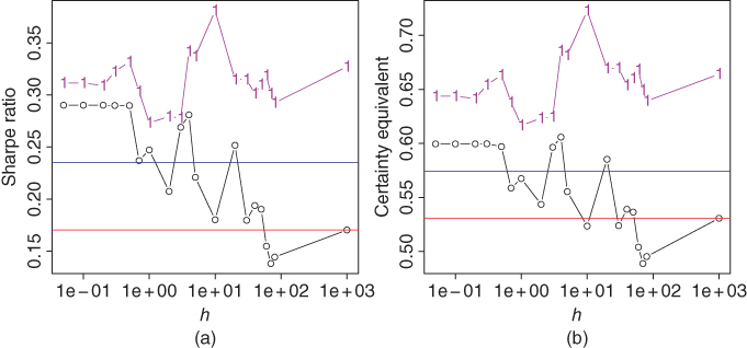
Figure 12.5 Trend following with moving averages. (a) Sharpe ratios of trend following strategies with S&P 500 (black curve) and 10-year bond (purple curve); (b) certainty equivalent is shown for the same portfolios as in panel (a). The  -axis shows the smoothing parameter of the moving average. The red horizontal line shows the Sharpe ratio of S&P 500 and the blue horizontal line shows the Sharpe ratio of 10-year bond.
Figure 12.6 shows the time series of the ratios of the cumulative wealth of a trend following strategy to the cumulative wealth of the benchmark. In panel (a) we follow the trend of S&P 500 and the benchmark is S&P 500. In panel (b) we follow the trend of US Treasury 10-year bond and the benchmark is US Treasury 10-year bond. The smoothing parameters of moving averages are ![]() (black),
(black), ![]() (red),
(red), ![]() (blue), and
(blue), and ![]() (green). For S&P 500 the smallest smoothing parameter gives the best result, but for 10-year bond a larger smoothing parameter gives the best result.
(green). For S&P 500 the smallest smoothing parameter gives the best result, but for 10-year bond a larger smoothing parameter gives the best result.
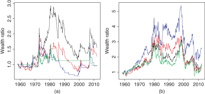
Figure 12.6 Trend following with moving averages: Wealth ratios. (a) Following the trend of S&P 500 and (b) following the trend of 10-year bond. We show the ratios of the cumulative wealth to cumulative wealth of the benchmark. The smoothing parameters of moving averages are  (black),
  (red),
  (blue), and
  (green).
12.3.1.3 Regression on Economic Indicators
We consider a portfolio strategy where the expected return of the risky asset is estimated,2 and if the estimated expected return is larger than the risk-free rate, then the weight of the risky asset is one, and the weight of the risk-free rate is zero. Otherwise, the weight of the risky asset is zero and the weight of the risk-free rate is one. The expected returns are estimated using linear regression on economic indicators, as explained in Section 6.4. Both dividend yield and term spread are used as predicting variables.
Figure 12.7 shows the Sharpe ratios as a function of the prediction horizon ![]() . Note that we predict 1-month returns, but the 1-month return predictions are deduced from a prediction with horizon
. Note that we predict 1-month returns, but the 1-month return predictions are deduced from a prediction with horizon ![]() . Panel (a) uses the prediction method of (6.35), and panel (b) uses the prediction method of (6.36). We can see that the Sharpe ratios of portfolios with 10-year bond are highest for short prediction horizons, whereas the Sharpe ratios of portfolios with S&P 500 are highest for the long prediction horizons.
. Panel (a) uses the prediction method of (6.35), and panel (b) uses the prediction method of (6.36). We can see that the Sharpe ratios of portfolios with 10-year bond are highest for short prediction horizons, whereas the Sharpe ratios of portfolios with S&P 500 are highest for the long prediction horizons.

Figure 12.7 Expected returns determined by economic indicators: Sharpe ratios. Sharpe ratios of portfolios with S&P 500 (black curve) and 10-year bond (purple curve). (a) The prediction method of (6.35) and (b) the prediction method of (6.36). The  -axis shows the prediction horizon. The red horizontal line shows the Sharpe ratio of S&P 500 and the blue horizontal line shows the Sharpe ratio of 10 year bond.
Figure 12.8 shows the cumulative wealth of the portfolios whose weights are chosen according to the expected returns. We use 12-month prediction horizon, so that ![]() in (6.34). Panel (a) shows the wealth on the
in (6.34). Panel (a) shows the wealth on the ![]() -axis and panel (b) uses logarithmic scale on the
-axis and panel (b) uses logarithmic scale on the ![]() -axis. The purple curves show the portfolio using 10-year bond as the risky asset, and the black curves show the portfolio using S&P 500 as the risky asset. The red curves show the cumulative wealth of S&P 500 and the blue curves show the cumulative wealth of 10-year bond. The wealth is normalized to have value one at the beginning. We can note that trend following increases the cumulative wealth, when compared to S&P 500 index and to 10-year bond. The linear segments in the black curves indicate that during these periods the risk-free investment is chosen.
-axis. The purple curves show the portfolio using 10-year bond as the risky asset, and the black curves show the portfolio using S&P 500 as the risky asset. The red curves show the cumulative wealth of S&P 500 and the blue curves show the cumulative wealth of 10-year bond. The wealth is normalized to have value one at the beginning. We can note that trend following increases the cumulative wealth, when compared to S&P 500 index and to 10-year bond. The linear segments in the black curves indicate that during these periods the risk-free investment is chosen.

Figure 12.8 Expected returns determined by economic indicators: Cumulative wealth. (a) The cumulative wealth of the portfolio whose weights are chosen according to the expected returns, when the risky asset is 10-year bond (purple) and S&P 500 (black); (b) logarithmic scale. The red curves show the cumulative wealth of S&P 500 and the blue curves show the wealth of 10-year bond.
Figure 12.9 considers the same strategies as in Figure 12.8 but now we show wealth ratios. Panel (a) shows the ratio of the wealth of trend following with S&P 500 to the wealth of S&P 500 (black) and the ratio of the wealth of trend following with 10-year bond to the wealth of 10-year bond (purple). Panel (b) shows the ratio of the wealth of trend following with S&P 500 to the wealth of trend following with 10-year bond. Figure 12.2 shows the corresponding time series for 1-month trend following. We see that using economic indicators improves the trading with S&P 500, whereas 1-month trend following works better when trading with 10-year bond.

Figure 12.9 Expected returns determined by economic indicators: Wealth ratios. (a) The ratio of the wealth of trend following with S&P 500 to the wealth of S&P 500 (black), and the ratio of the wealth of trend following with 10-year bond to the wealth of 10-year bond (purple); (b) The ratio of the wealth of trend following with S&P 500 to the wealth of trend following with 10-year bond.
12.3.2 Markowitz Portfolios with One Risky Asset
Variance penalization with the risk-free rate was discussed in Section 11.1.1. Using this approach, when there is one risky asset and the risk aversion is ![]() , we maximize
, we maximize
over ![]() , where
, where ![]() is the expected gross return of the risky asset,
is the expected gross return of the risky asset, ![]() is the risk-free rate, and
is the risk-free rate, and ![]() is the variance of the return of the risky asset. The maximizer was given in (11.3) as
is the variance of the return of the risky asset. The maximizer was given in (11.3) as
When the maximization is restricted to ![]() , then the solution was given in (11.4) as
, then the solution was given in (11.4) as

We estimate the expected return using either moving averages or regression on economic indicators. The variance is estimated always using moving averages, which contains the sequentially computed sample variance as a special case. Variance estimation with moving averages is studied in Section 7.4.
12.3.2.1 Using Moving Averages
Figure 12.10 extends the approach of Figure 12.5. The expected return is again estimated using an exponentially weighted moving average, but now the weight of the risky asset is chosen as in (12.20). Variance ![]() is the additional parameter to be estimated. Panel (a) shows the Sharpe ratios as a function of the smoothing parameter
is the additional parameter to be estimated. Panel (a) shows the Sharpe ratios as a function of the smoothing parameter ![]() of the moving average, which estimates the expected return. The variance is estimated by the sequentially calculated sample variance. We can see that the Sharpe ratio of the portfolio with S&P 500 as the risky asset is highest for smaller smoothing parameters, whereas the Sharpe ratio of the strategy with 10-year bond as the risky asset has a high level for all smoothing parameters. Panel (b) shows a contour plot: we show Sharpe ratio both as a function of the smoothing parameter of the moving average for the estimation of the expected return
of the moving average, which estimates the expected return. The variance is estimated by the sequentially calculated sample variance. We can see that the Sharpe ratio of the portfolio with S&P 500 as the risky asset is highest for smaller smoothing parameters, whereas the Sharpe ratio of the strategy with 10-year bond as the risky asset has a high level for all smoothing parameters. Panel (b) shows a contour plot: we show Sharpe ratio both as a function of the smoothing parameter of the moving average for the estimation of the expected return ![]() (
(![]() -axis), and as a function of the moving average for the estimation of volatility
-axis), and as a function of the moving average for the estimation of volatility ![]() (
(![]() -axis), when the portfolio has S&P 500 index as the risky asset.3 We can see that the smoothing parameter of the volatility estimate has hardly any influence on the Sharpe ratio, and only the smoothing parameter of the estimate of the expected return has an influence.
-axis), when the portfolio has S&P 500 index as the risky asset.3 We can see that the smoothing parameter of the volatility estimate has hardly any influence on the Sharpe ratio, and only the smoothing parameter of the estimate of the expected return has an influence.

Figure 12.10 Markowitz portfolios with moving averages: Sharpe ratios. (a) Sharpe ratios of trend following strategies with S&P 500 (black curve) and 10-year bond (purple curve). The  -axis shows the smoothing parameter of the moving average. The red horizontal line shows the Sharpe ratio of S&P 500 and the blue horizontal line shows the Sharpe ratio of 10 year bond. (b) Sharpe ratios of trend following strategies with S&P 500 when both expected returns and volatility are estimated using moving averages.
Figure 12.11 shows wealth ratios of Markowitz strategies when the expected returns are estimated using moving averages and the variances are estimated using sequential sample variances. Panel (a) shows trading with S&P 500 and panel (b) shows trading with 10-year bond. The wealth of Markowitz strategies is divided by the benchmark (S&P 500 index in (a) and 10-year bond in (b)). The smoothing parameters of moving averages are ![]() (black),
(black), ![]() (red),
(red), ![]() (blue), and
(blue), and ![]() (green). Note that Figure 12.6 shows the corresponding time series for the case where the variance is ignored. The Markowitz criterion does not seem to improve the wealth ratios, when compared to the simple trend following.
(green). Note that Figure 12.6 shows the corresponding time series for the case where the variance is ignored. The Markowitz criterion does not seem to improve the wealth ratios, when compared to the simple trend following.

Figure 12.11 Markowitz portfolios with moving averages: Wealth ratios. (a) Trading with S&P 500 and (b) trading with 10-year bond. We show the ratios of the cumulative wealth to cumulative wealth of the benchmark. The smoothing parameters of moving averages are  (black),
  (red),
  (blue), and
  (green).
Figure 12.12 studies the effect of relaxing the restrictions on short selling and leveraging. Figure 12.10 studies the case where short selling and leveraging are not allowed. More generally, we can restrict the maximization in (12.18) to ![]() , where
, where ![]() . The weight that maximizes the Markowitz criterion is given by
. The weight that maximizes the Markowitz criterion is given by

where ![]() is defined in (12.19). Figure 12.12 shows Sharpe ratios of the portfolio as a function of smoothing parameter
is defined in (12.19). Figure 12.12 shows Sharpe ratios of the portfolio as a function of smoothing parameter ![]() when (a) the risky asset is S&P 500 index and (b) the risky asset is 10-year bond. The lines with label “1” show the case when
when (a) the risky asset is S&P 500 index and (b) the risky asset is 10-year bond. The lines with label “1” show the case when ![]() (these are the same lines as in Figure 12.10(a)). The lines with label “2” show the case when
(these are the same lines as in Figure 12.10(a)). The lines with label “2” show the case when ![]() , and the lines with label “3” show the case when
, and the lines with label “3” show the case when ![]() . We can see that the Sharpe ratios are decreasing when more short selling and leveraging are allowed.
. We can see that the Sharpe ratios are decreasing when more short selling and leveraging are allowed.

Figure 12.12 Markowitz portfolios with moving averages: Sharpe ratios when short selling and leveraging are allowed. Sharpe ratios of trend following strategies as a function of smoothing parameter  when the risky asset is (a) S&P 500; (b) 10-year bond. The red horizontal line show the Sharpe ratio of S&P 500 and the blue horizontal line show the Sharpe ratio of 10 year bond.
12.3.2.2 Using Economic Indicators
Figure 12.13 shows the Sharpe ratios as a function of the prediction horizon ![]() (in months). Note that we predict 1-month returns, and use the prediction horizon
(in months). Note that we predict 1-month returns, and use the prediction horizon ![]() in the construction of 1-month predictions. We use the Markowitz weight (12.20), estimate the expected return using linear regression on dividend yield and term spread, and estimate the variance with the sequential standard deviation. Panel (a) uses the prediction method of (6.35) and and panel (b) uses the prediction method of (6.36). The black curves show the cases where the risky asset is S&P 500 and the purple curves show the cases where the risky asset is the US 10-year bond. The blue horizontal lines show the Sharpe ratio of S&P 500 and the red horizontal lines show the Sharpe ratio of 10-year bond. Similar to Figure 12.7, we can see that the Sharpe ratios of portfolios with 10-year bond are highest for short prediction horizons, whereas the Sharpe ratios of portfolios with S&P 500 are highest for the long prediction horizons.
in the construction of 1-month predictions. We use the Markowitz weight (12.20), estimate the expected return using linear regression on dividend yield and term spread, and estimate the variance with the sequential standard deviation. Panel (a) uses the prediction method of (6.35) and and panel (b) uses the prediction method of (6.36). The black curves show the cases where the risky asset is S&P 500 and the purple curves show the cases where the risky asset is the US 10-year bond. The blue horizontal lines show the Sharpe ratio of S&P 500 and the red horizontal lines show the Sharpe ratio of 10-year bond. Similar to Figure 12.7, we can see that the Sharpe ratios of portfolios with 10-year bond are highest for short prediction horizons, whereas the Sharpe ratios of portfolios with S&P 500 are highest for the long prediction horizons.

Figure 12.13 Sharpe ratios as a function of prediction horizon when the expected returns are determined by economic indicators: Markowitz criterion. Sharpe ratios of portfolios with S&P 500 (black curve) and 10-year bond (purple curve). (a) The prediction method of (6.35) and (b) the prediction method of (6.36). The  -axis shows the prediction horizon. The red horizontal line shows the Sharpe ratio of S&P 500 and the blue horizontal line shows the Sharpe ratio of 10 year bond.
12.4 Two Risky Assets
Section 12.4.1 studies portfolio selection using only prediction of the returns and Section 12.4.2 studies the use of the Markowitz mean–variance criterion.
12.4.1 Using Expected Returns with Two Risky Assets
We study portfolio selection that uses only the expected returns to choose the weights (risk aversion is zero). This means that when the expected return of the bond is larger than the expected return of the stock, then everything is invested in the bond, and conversely.
We consider portfolio strategies where the portfolio weight is chosen solely on the basis of expected returns. We call trend following strategies such strategies, where the expected return is estimated solely on the basis of previous returns, by guessing that the near future is similar to the near past. However, expected returns can also be estimated by using regression on economic indicators and by using regression on previous returns.
12.4.1.1 One Step Trend Following
We have two risky assets and consider the decision rule that invests everything in the first asset if the previous period return of the first asset was bigger than the previous period return of the second asset. Otherwise, the second asset is chosen. Let us denote
where ![]() and
and ![]() are the gross returns of assets 1 and 2. Let the weight of the first asset be
are the gross returns of assets 1 and 2. Let the weight of the first asset be ![]() if
if ![]() and otherwise
and otherwise ![]() .
.
Figure 12.14 shows the cumulative wealth of the trend following portfolios. Panel (a) shows the wealth on the ![]() -axis and panel (b) uses logarithmic scale on the
-axis and panel (b) uses logarithmic scale on the ![]() -axis. The black curves show the actively managed portfolio. The red curves show the cumulative wealth of S&P 500 and the blue curves show the wealth of 10-year bond. The wealth is normalized to be one at the beginning. We can note that the trend following increases the cumulative wealth, when compared to S&P 500 index or 10-year bond.
-axis. The black curves show the actively managed portfolio. The red curves show the cumulative wealth of S&P 500 and the blue curves show the wealth of 10-year bond. The wealth is normalized to be one at the beginning. We can note that the trend following increases the cumulative wealth, when compared to S&P 500 index or 10-year bond.

Figure 12.14 Trend following with the previous 1-month return and two risky assets: Cumulative wealth. (a) The cumulative wealth of the trend following portfolio (black); (b) logarithmic scale. The red curves show the cumulative wealth of S&P 500 and the blue curves show the wealth of 10-year bond.
Figure 12.15 shows the ratios of cumulative wealth of the trend following portfolio. Panel (a) compares the trend following to the two benchmarks and panel (b) compares the two asset trend following to the two possible one asset trend following strategies. The one asset trend following is studied in Figures 12.1–12.4. In panel (a) the wealth of the two asset trend following is divided by the S&P 500 wealth (dark green) and 10-year bond wealth (orange). In panel (b) the wealth of the two asset trend following is divided by the wealth of S&P 500 trend following (dark green) and the wealth of 10-year bond trend following (orange). Panel (a) shows that the two asset trend following performs better than the two benchmarks in the most time periods. Panel (b) shows that the one asset trend following is better until 1980, but after that the two asset trend following is better.
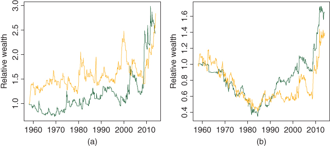
Figure 12.15 Trend following with the previous 1-month return and two risky assets: Wealth ratios. (a) The wealth of the two asset trend following is divided by the S&P 500 wealth (dark green) and 10-year bond wealth (orange); (b) the wealth of the two asset trend following is divided by the wealth of S&P 500 trend following (dark green) and the wealth of 10-year bond trend following (orange).
12.4.1.2 Trend Following with Moving Averages
Figure 12.16 considers generalization of the simple 1-month trend following shown in Figure 12.1. We define trend following with a moving average so that if a moving average of the returns of the first risky asset is larger than the moving average of the second risky asset, then the weight of the first risky asset is one and the weight of the second risky asset is zero. Otherwise, the weight of the first risky asset is zero and the weight of the second risky asset is one. We use the exponential moving average, defined in (6.7). The 1-month trend following strategy of Figure 12.14 is obtained as a special case by choosing the window of the moving average so small that the moving average is equal to the previous 1-month return.
Figure 12.16 shows (a) the Sharpe ratios and (b) the certainty equivalents4 of the moving average strategy as a function of the smoothing parameter ![]() of the moving average. We can see that the performance measures of trend following with moving averages are highest for smaller smoothing parameters. When the smoothing parameter becomes larger, then the Sharpe ratio of trend following with S&P 500 converges to the Sharpe ratio of S&P 500 index. This is because trend following with S&P 500 and with a large smoothing parameter chooses always to invest to S&P 500 and never to the risk-free rate. For the trend following with 10-year bond the convergence toward the performance measure of the underlying 10-year bond does not happen, because a moving average even with a large smoothing parameter is smaller than the risk-free rate during time periods before 1980s.
of the moving average. We can see that the performance measures of trend following with moving averages are highest for smaller smoothing parameters. When the smoothing parameter becomes larger, then the Sharpe ratio of trend following with S&P 500 converges to the Sharpe ratio of S&P 500 index. This is because trend following with S&P 500 and with a large smoothing parameter chooses always to invest to S&P 500 and never to the risk-free rate. For the trend following with 10-year bond the convergence toward the performance measure of the underlying 10-year bond does not happen, because a moving average even with a large smoothing parameter is smaller than the risk-free rate during time periods before 1980s.

Figure 12.16 Trend following with moving averages. (a) Sharpe ratios of trend following strategies (black curve); (b) certainty equivalent is shown for the same portfolios as in panel (a). The  -axis shows the smoothing parameter of the moving average. The red horizontal line shows the Sharpe ratio of S&P 500 and the blue horizontal line shows the Sharpe ratio of 10 year bond.
12.4.1.3 Regression on Economic Indicators
We consider a portfolio strategy where the expected returns of the risky assets are estimated, and if the estimated expected return of the first asset is larger than the estimated expected return of the second asset, then the weight of the first asset is one, and the weight of the second asset is zero. Otherwise, the weight of the first asset is zero, and the weight of the second asset is one. The expected returns are estimated using linear regression on economic indicators, as explained in Section 6.4. Both dividend yield and term spread are used as the predicting variables.
Figure 12.17 shows the Sharpe ratios as a function of the prediction horizon. Panel (a) uses the prediction method of (6.35) and and panel (b) uses the prediction method of (6.36). The two prediction methods seem to lead similar performances. The prediction horizon about ![]() gives the best results. Note that we are making predictions of 1-month returns, but the predictions are constructed with the help of predictions with horizon
gives the best results. Note that we are making predictions of 1-month returns, but the predictions are constructed with the help of predictions with horizon ![]() .
.
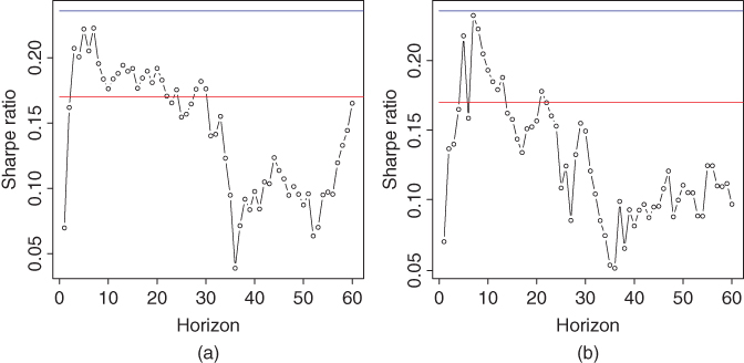
Figure 12.17 Expected returns determined by economic indicators: Sharpe ratios. Sharpe ratios of managed portfolios. (a) The prediction method of (6.35) and (b) the prediction method of (6.36). The  -axis shows the prediction horizon. The red horizontal line shows the Sharpe ratio of S&P 500 and the blue horizontal line shows the Sharpe ratio of 10 year bond.
Figure 12.18 shows the cumulative wealth of the portfolio whose weights are chosen according to the expected returns. Panel (a) shows the wealth on the ![]() -axis and panel (b) uses logarithmic scale on the
-axis and panel (b) uses logarithmic scale on the ![]() -axis. The prediction horizon is
-axis. The prediction horizon is ![]() months. The prediction method of (6.35) is used. The black curves show the actively managed portfolio. The red curves show the cumulative wealth of S&P 500 and the blue curves show the cumulative wealth of 10-year bond.
months. The prediction method of (6.35) is used. The black curves show the actively managed portfolio. The red curves show the cumulative wealth of S&P 500 and the blue curves show the cumulative wealth of 10-year bond.
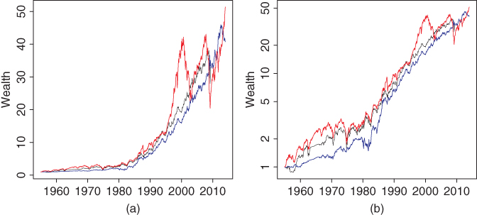
Figure 12.18 Expected returns determined by economic indicators: Cumulative wealth. (a) The cumulative wealth of the portfolio whose weights are chosen according to the expected return (black); (b) logarithmic scale. The red curves show the cumulative wealth of S&P 500 and the blue curves show the wealth of 10-year bond. The wealth is normalized to have value one at the beginning.
12.4.2 Markowitz Portfolios with Two Risky Assets
Variance penalization without a risk-free rate is discussed in Section 11.1.2. In this approach, when there are two risky assets and the risk aversion is ![]() , we maximize
, we maximize
over ![]() , where
, where ![]() and
and ![]() are the expected gross returns of the risky assets,
are the expected gross returns of the risky assets, ![]() and
and ![]() are the variances of the returns of the risky assets, and
are the variances of the returns of the risky assets, and ![]() is the covariance between the returns of the risky assets. The maximizer was given in (11.6) as
is the covariance between the returns of the risky assets. The maximizer was given in (11.6) as

When the maximization is restricted to ![]() , then the solution was given in (11.7) as
, then the solution was given in (11.7) as

12.4.2.1 Moving Averages
The means, variances, and the covariance in (12.22) are estimated using the exponentially weighted moving averages. The smoothing parameter ![]() is interpreted as the sequential sample mean, variance, or covariance. Thus, we have up to five smoothing parameters to choose. However, we use always the same smoothing parameter for the two means, and the same smoothing parameter for the two variances. So, we have three smoothing parameters to choose.
is interpreted as the sequential sample mean, variance, or covariance. Thus, we have up to five smoothing parameters to choose. However, we use always the same smoothing parameter for the two means, and the same smoothing parameter for the two variances. So, we have three smoothing parameters to choose.
Figure 12.19 shows Sharpe ratios as a function of smoothing parameters. The weight of the second risky asset is chosen as in (12.23). The means and variances are estimated with the exponentially weighted moving averages, and the covariance is the sequential sample covariance. Panel (a) shows the Sharpe ratios as a function of the smoothing parameter of the means ![]() and
and ![]() , for the smoothing parameters of the variance in the range 1–1000. Panel (b) shows the Sharpe ratios as a function of the smoothing parameter of the variances
, for the smoothing parameters of the variance in the range 1–1000. Panel (b) shows the Sharpe ratios as a function of the smoothing parameter of the variances ![]() and
and ![]() , for the smoothing parameters of the means in the range 0.1–1000. The labels “1”–“6” and “1”–“5” correspond to the smoothing parameters in the increasing order. We can see that the Sharpe ratio of the portfolio is highest for the smallest smoothing parameters of the estimator of the expected return, but the variances require a large smoothing parameter.
, for the smoothing parameters of the means in the range 0.1–1000. The labels “1”–“6” and “1”–“5” correspond to the smoothing parameters in the increasing order. We can see that the Sharpe ratio of the portfolio is highest for the smallest smoothing parameters of the estimator of the expected return, but the variances require a large smoothing parameter.

Figure 12.19 Markowitz portfolios with two risky assets and moving averages: Sharpe ratios. (a) Sharpe ratios as a function of the smoothing parameter of the means  and
and  , for the smoothing parameter of the variances in the range 1–1000; (b) Sharpe ratios as a function of the smoothing parameter of the variances
  and
and  , for the smoothing parameter of the means in the range 0.1–1000.
Figure 12.20 shows Sharpe ratios as a function of smoothing parameters. The weight of the second risky asset is chosen as in (12.23). The means, variances, and the covariances are estimated with the exponentially weighted moving averages. The smoothing parameter of the estimator of the means is ![]() . Panel (a) shows the Sharpe ratios as a function of the smoothing parameter of the variances
. Panel (a) shows the Sharpe ratios as a function of the smoothing parameter of the variances ![]() and
and ![]() , for the smoothing parameters of the covariance in the range 1–1000. Panel (b) shows the Sharpe ratios as a function of the smoothing parameter of the covariance
, for the smoothing parameters of the covariance in the range 1–1000. Panel (b) shows the Sharpe ratios as a function of the smoothing parameter of the covariance ![]() , for the smoothing parameters of the variances in the range 1–1000. The labels “1”–“5” correspond to the smoothing parameters in the increasing order. The Sharpe ratio of S&P 500 is shown with a red horizontal line, and the Sharpe ratio of 10 year bond is shown with a blue horizontal line. We can see that a large Sharpe ratio is obtained when the both smoothing parameters are about
, for the smoothing parameters of the variances in the range 1–1000. The labels “1”–“5” correspond to the smoothing parameters in the increasing order. The Sharpe ratio of S&P 500 is shown with a red horizontal line, and the Sharpe ratio of 10 year bond is shown with a blue horizontal line. We can see that a large Sharpe ratio is obtained when the both smoothing parameters are about ![]() .
.

Figure 12.20 Markowitz portfolios with two risky assets and moving averages: Sharpe ratios. (a) Sharpe ratios as a function of the smoothing parameter of the variances  and
and  , for the smoothing parameter of the covariance in the range 1–1000; (b) Sharpe ratios as a function of the smoothing parameter of the covariance
  , for the smoothing parameter of the variances in the range 1–1000.
Figure 12.21 studies the effect of relaxing the restrictions on short selling and leveraging, whereas in Figure 12.19 short selling and leveraging are not allowed. Now, we restrict the maximization in (12.21) to ![]() , where
, where ![]() . The maximizing weight is
. The maximizing weight is

where ![]() is defined in (12.22). Figure 12.21 shows Sharpe ratios as a function of smoothing parameters. The means and variances are estimated with the exponentially weighted moving averages, and the covariance is the sequential sample covariance. Panel (a) shows the Sharpe ratios as a function of the smoothing parameter of the means
is defined in (12.22). Figure 12.21 shows Sharpe ratios as a function of smoothing parameters. The means and variances are estimated with the exponentially weighted moving averages, and the covariance is the sequential sample covariance. Panel (a) shows the Sharpe ratios as a function of the smoothing parameter of the means ![]() and
and ![]() , for the smoothing parameter of the variances equal to 1000. Panel (b) shows the Sharpe ratios as a function of the smoothing parameter of the variances
, for the smoothing parameter of the variances equal to 1000. Panel (b) shows the Sharpe ratios as a function of the smoothing parameter of the variances ![]() and
and ![]() , for the smoothing parameter of the means equal to 0.1. The lines with label “1” show the case when
, for the smoothing parameter of the means equal to 0.1. The lines with label “1” show the case when ![]() (these are the same lines as in Figure 12.19). The lines with label “2” show the case when
(these are the same lines as in Figure 12.19). The lines with label “2” show the case when ![]() and the lines with label “3” show the case when
and the lines with label “3” show the case when ![]() . The red horizontal line shows the Sharpe ratio of S&P 500 and the blue horizontal line shows the Sharpe ratio of 10-year bond. We can see that the Sharpe ratios are smaller when more short selling and leveraging are allowed.
. The red horizontal line shows the Sharpe ratio of S&P 500 and the blue horizontal line shows the Sharpe ratio of 10-year bond. We can see that the Sharpe ratios are smaller when more short selling and leveraging are allowed.

Figure 12.21 Markowitz portfolios with two risky assets: Moving averages when short selling and leveraging are allowed. (a) Sharpe ratios as a function of the smoothing parameter of the means  and
and  ; (b) Sharpe ratios as a function of the smoothing parameter of the variances
  and
and  . The curve with labels “1”
  leverage, labels “2” indicate leverage
  , and labels “3” indicate leverage
  . The red horizontal line shows the Sharpe ratio of S&P 500 and the blue horizontal line shows the Sharpe ratio of 10-year bond.
Figure 12.22 shows wealth and relative wealth. The smoothing parameter of the estimators of the expected returns is ![]() , for the variances and the covariance
, for the variances and the covariance ![]() . Panel (a) shows the cumulative wealth of the Markowitz portfolio (black), S&P 500 (red), and 10-year bond (blue). Panel (b) shows the ratios of the wealth of the Markowitz portfolio to the wealth of S&P 500 (purple) and to the wealth of 10-year bond (orange). The wealth is normalized to have value one at the beginning. Panel (a) shows that the Markowitz portfolio beats the benchmarks. Panel (b) shows that the Markowitz portfolio beats the benchmarks during the most time periods.
. Panel (a) shows the cumulative wealth of the Markowitz portfolio (black), S&P 500 (red), and 10-year bond (blue). Panel (b) shows the ratios of the wealth of the Markowitz portfolio to the wealth of S&P 500 (purple) and to the wealth of 10-year bond (orange). The wealth is normalized to have value one at the beginning. Panel (a) shows that the Markowitz portfolio beats the benchmarks. Panel (b) shows that the Markowitz portfolio beats the benchmarks during the most time periods.

Figure 12.22 Markowitz portfolios with two risky assets and moving averages: Wealth. (a) The cumulative wealth of the Markowitz portfolio (black), S&P 500 (red), and 10-year bond (blue); (b) the ratios of the wealth of the Markowitz portfolio to the wealth of S&P 500 (purple) and to the wealth of 10-year bond (orange).
12.4.2.2 Using Economic Indicators
We use the Markowitz weight (12.23). The means are estimated using linear regression on dividend yield and term spread. The two methods of linear regression are defined in (6.35) and (6.36). The variances and the covariance are estimated with exponentially weighted moving averages. The smoothing parameter ![]() is interpreted as the sequential sample variance or covariance. Thus, we have up to five parameters to choose: two horizon parameters
is interpreted as the sequential sample variance or covariance. Thus, we have up to five parameters to choose: two horizon parameters ![]() for the estimation of the two means, two smoothing parameters
for the estimation of the two means, two smoothing parameters ![]() for the two variances, and one smoothing parameter
for the two variances, and one smoothing parameter ![]() to estimate the covariance. However, we use always the same horizon parameter for the two means, and the same smoothing parameter for the two variances. So, we have three parameters to choose.
to estimate the covariance. However, we use always the same horizon parameter for the two means, and the same smoothing parameter for the two variances. So, we have three parameters to choose.
Figure 12.23 shows the Sharpe ratios of the Markowitz portfolios. The prediction method of (6.35) is used. The covariance is estimated by the sequential sample covariance. Panel (a) shows the Sharpe ratios as a function of the parameter ![]() of the prediction horizon, for values
of the prediction horizon, for values ![]() –1000 of the smoothing parameter of the estimator of the variances. The symbols “1”–“4” correspond to the smoothing parameters of the variances in the increasing order. Panel (b) shows the Sharpe ratios as a function of the smoothing parameter of the estimator of the variances, for prediction horizons
–1000 of the smoothing parameter of the estimator of the variances. The symbols “1”–“4” correspond to the smoothing parameters of the variances in the increasing order. Panel (b) shows the Sharpe ratios as a function of the smoothing parameter of the estimator of the variances, for prediction horizons ![]() –120. Panel (a) shows that the prediction horizon around
–120. Panel (a) shows that the prediction horizon around ![]() gives the largest Sharpe ratio. Panel (b) shows that the smoothing parameter of the estimator of the variances should not be too small.
gives the largest Sharpe ratio. Panel (b) shows that the smoothing parameter of the estimator of the variances should not be too small.

Figure 12.23 Regression on economic indicators: Sharpe ratios. (a) Sharpe ratios as a function of the prediction horizon, for values  –1000 of the smoothing parameter of the variances; (b) Sharpe ratios as a function of the smoothing parameter of the variances, for prediction horizons
  –120.
–120.
Figure 12.24 compares the two methods (6.35) and (6.36) of linear regression. The Sharpe ratios of (6.35) are divided by the Sharpe ratios of (6.36). Panel (a) shows the ratios of the Sharpe ratios as a function of the parameter ![]() of the prediction horizon, for values
of the prediction horizon, for values ![]() –1000 of the smoothing parameter of the estimator of the variances. Panel (b) shows the ratios of the Sharpe ratios as a function of the smoothing parameter of the estimator of the variances, for prediction horizons
–1000 of the smoothing parameter of the estimator of the variances. Panel (b) shows the ratios of the Sharpe ratios as a function of the smoothing parameter of the estimator of the variances, for prediction horizons ![]() –120. We see that the ratios of the Sharpe ratios are smaller than one: the Sharpe ratios of (6.36) are larger than the Sharpe ratios of (6.35).
–120. We see that the ratios of the Sharpe ratios are smaller than one: the Sharpe ratios of (6.36) are larger than the Sharpe ratios of (6.35).

Figure 12.24 Regression on economic indicators: Ratios of the Sharpe ratios. The Sharpe ratios of (6.35) are divided by the Sharpe ratios of (6.36). (a) The ratios as a function of the prediction horizon, for values  –1000 of the smoothing parameter of the variances; (b) the ratios as a function of the smoothing parameter of the variances, for prediction horizons
  –120.
–120.
Figure 12.25 shows the Sharpe ratios of the Markowitz portfolios. The prediction method of (6.35) is used. The prediction horizon of the expected returns is ![]() . Panel (a) shows the Sharpe ratios as a function of the smoothing parameter of the estimator of the variances, for values
. Panel (a) shows the Sharpe ratios as a function of the smoothing parameter of the estimator of the variances, for values ![]() –1000 of the smoothing parameter of the covariance. Panel (b) shows the Sharpe ratios as a function of the smoothing parameter of the estimator of the covariance, for values
–1000 of the smoothing parameter of the covariance. Panel (b) shows the Sharpe ratios as a function of the smoothing parameter of the estimator of the covariance, for values ![]() –1000 of the smoothing parameter of the variances. The symbols “1”–“4” correspond the smoothing parameters in the increasing order. The red horizontal lines show the Sharpe ratio of S&P 500 and the blue horizontal lines show the Sharpe ratio of 10-year bond. Panel (a) shows that the smoothing parameter of the variances should be large, especially when the smoothing parameter of the covariance is small. Panel (b) shows that when the smoothing parameter of the variances is large, then the smoothing parameter of the covariance should be small.
–1000 of the smoothing parameter of the variances. The symbols “1”–“4” correspond the smoothing parameters in the increasing order. The red horizontal lines show the Sharpe ratio of S&P 500 and the blue horizontal lines show the Sharpe ratio of 10-year bond. Panel (a) shows that the smoothing parameter of the variances should be large, especially when the smoothing parameter of the covariance is small. Panel (b) shows that when the smoothing parameter of the variances is large, then the smoothing parameter of the covariance should be small.

Figure 12.25 Regression on economic indicators: Sharpe ratios. (a) The Sharpe ratios as a function of the smoothing parameter of the estimator of the variances, for values  –1000 of the smoothing parameter of the covariance; (b) the Sharpe ratios as a function of the smoothing parameter of the estimator of the covariance, for values
  –1000 of the smoothing parameter of the variances.
Figure 12.26 is otherwise similar to Figure 12.25, but now the the prediction method of (6.36) is used, instead of the prediction method of (6.35).

Figure 12.26 Regression on economic indicators: Sharpe ratios of method (6.36). (a) The Sharpe ratios as a function of the smoothing parameter of the estimator of the variances, for values  –1000 of the smoothing parameter of the covariance; (b) the Sharpe ratios as a function of the smoothing parameter of the estimator of the covariance, for values
  –1000 of the smoothing parameter of the variances.
Figure 12.27 shows wealth and relative wealth. The prediction horizon of the estimator of the expected return is ![]() . The prediction method of (6.35) is used. The smoothing parameter of the variances is
. The prediction method of (6.35) is used. The smoothing parameter of the variances is ![]() , and the smoothing parameter of the covariance is
, and the smoothing parameter of the covariance is ![]() . Panel (a) shows the cumulative wealth of the Markowitz portfolio (black), S&P 500 (red), and 10-year bond (blue). Panel (b) shows the ratios of the wealth of the Markowitz portfolio to the wealth of S&P 500 (purple) and to the wealth of 10-year bond (orange). The wealth is normalized to have value one at the beginning. Panel (a) shows that the Markowitz portfolio beats the benchmarks. Panel (b) shows that the Markowitz portfolio beats the benchmarks during the most time periods, and the performance of the Markowitz portfolio is close to the performance of the 10-year bond after about 1985.
. Panel (a) shows the cumulative wealth of the Markowitz portfolio (black), S&P 500 (red), and 10-year bond (blue). Panel (b) shows the ratios of the wealth of the Markowitz portfolio to the wealth of S&P 500 (purple) and to the wealth of 10-year bond (orange). The wealth is normalized to have value one at the beginning. Panel (a) shows that the Markowitz portfolio beats the benchmarks. Panel (b) shows that the Markowitz portfolio beats the benchmarks during the most time periods, and the performance of the Markowitz portfolio is close to the performance of the 10-year bond after about 1985.

Figure 12.27 Regression on economic indicators: Wealth. (a) The cumulative wealth of the Markowitz portfolio (black), S&P 500 (red), and 10-year bond (blue); (b) the ratios of the wealth of the Markowitz portfolio to the wealth of S&P 500 (purple) and to the wealth of 10-year bond (orange).

Figure 12.28 Regression on economic indicators with the method (6.36): Wealth. (a) The cumulative wealth of the Markowitz portfolio (black), S&P 500 (red), and 10-year bond (blue); (b) the ratios of the wealth of the Markowitz portfolio to the wealth of S&P 500 (purple) and to the wealth of 10-year bond (orange).

Figure 12.29 Conditional versus unconditional estimation. (a) Time series of the portfolio wealth when the first and second moments are estimated conditionally (black), first moments sequentially and second moments conditionally (green), first moments conditionally and second moments sequentially (yellow), and first and second moments are estimated sequentially (purple); (b) relative wealths with respect to the wealth of S&P 500.
Figure 12.28 shows wealth and relative wealth. The prediction horizon of the estimator of the expected return is ![]() . The prediction method of (6.36) is used. The smoothing parameter of the variances is
. The prediction method of (6.36) is used. The smoothing parameter of the variances is ![]() , and the smoothing parameter of the covariance is
, and the smoothing parameter of the covariance is ![]() . Panel (a) shows the cumulative wealth of the Markowitz portfolio (black), S&P 500 (red), and 10-year bond (blue). Panel (b) shows the ratios of the wealth of the Markowitz portfolio to the wealth of S&P 500 (purple) and to the wealth of 10-year bond (orange). The wealth is normalized to have value one at the beginning. Panel (a) shows that the Markowitz portfolio beats the benchmarks, and the Markowitz portfolio of Figure 12.27. Panel (b) shows that the Markowitz portfolio beats the benchmarks during the most time periods.
. Panel (a) shows the cumulative wealth of the Markowitz portfolio (black), S&P 500 (red), and 10-year bond (blue). Panel (b) shows the ratios of the wealth of the Markowitz portfolio to the wealth of S&P 500 (purple) and to the wealth of 10-year bond (orange). The wealth is normalized to have value one at the beginning. Panel (a) shows that the Markowitz portfolio beats the benchmarks, and the Markowitz portfolio of Figure 12.27. Panel (b) shows that the Markowitz portfolio beats the benchmarks during the most time periods.
Figure 12.29 studies the importance of conditional prediction of second moments. Panel (a) shows the wealths and panel (b) shows the relative wealths with respect to the wealth of S&P 500. The black curve is the same as in Figure 12.28, so that both the expectations and the second moments are estimated conditionally. The green curve corresponds to the case where only the second moments are estimated conditionally but the returns are predicted sequentially. The yellow curve corresponds to the case where only the returns are predicted conditionally but the second moments are predicted sequentially. The purple curve corresponds to the case where both the expectations and the second moments are estimated sequentially. The wealth is normalized to have value one at the beginning. We see that the black and green curves are much better, so that the conditional expectation of the second moments is more important than the conditional estimation of the expectations.