Chapter 6: Auto Charts: Bulk Generation of Charts
About Auto Charts and Bulk Generation of Charts
Add an Axis Table to the Graph
About Auto Charts and Bulk Generation of Charts
In previous chapters of this book, you created a single graph and assigned data to the variables in plots. This process works well when you know the data and what type of graph you want. This is called a chart-centric approach.
But often, you get new data with new variables, and you don’t know what type of graph you need or what variable associations exist. In this case, it is useful to see how different variables look in a graph, including how combinations of variables look. This is called a data-centric approach. This chapter discusses an Auto Charts tool that generates graphs in bulk based on different variables.
The Auto Charts tool enables you to create graphs in bulk from a list of variables that you specify and using graph types that you select. Based on your selections, the Auto Charts tool uses a patent-pending process to create multiple graphs using various variable combinations. The tool shows you how many graphs it is going to generate, generates the graphs, and populates icons for each graph in the Auto Charts window. A progress bar is displayed, and the process can be interrupted or restarted at any time.
After generating the graphs, you can choose one or more graphs as a starting point. For example, you can modify the automatically generated titles and legends. You can add more plots and items to a graph. You can save the generated graph as an image file or in other formats, including a SAS ODS Graphics Designer (SGD) file that you can later edit.
The Auto Charts tool is ideal for exploring different visualizations of your data. You can generate a series of graphs, and then choose the ones that best display your information. If you are not satisfied with the graphs, you can change a few parameters and generate a whole new set of graphs.
The Auto Charts Window
You specify your data in the Auto Charts window, and the SAS ODS Graphics Designer (the designer) generates graphs for that data. The following figure shows an Auto Charts window that has been populated with sample data and automatically generated graphs:
Figure 6.1 Sample Auto Charts Window

The Auto Charts window has three main panes in which you can perform the following tasks:
Top pane
Specify the SAS library and data set for your graphs.
Left pane
Select one or more variables for your graphs. Specify the types of graphs that you want to generate. Generate graphs.
The top portion of the left pane is a table of variables. The columns contain the following information:
◦ Variable displays the name of each variable in the data set. To select a variable, select the variable’s check box.
◦ Details provides more information about the variable values. Character variables and discrete numeric variables display the value count for the variable. Continuous numeric variables display the range of the value. Variables that have a Type=Any setting display the count and the range.
◦ Type displays the data type. Data types include Continuous, Discrete, Time, and Any. The Any value enables the variable to apply to any of the data types that it supports. You can change the data type if a small triangle appears next to it.
The bottom portion of the left pane has four options for the types of graphs that you want to generate.
◦ Univariate and Bivariate are selected by default when you first open the Auto Charts window in a SAS session. You can clear either check box.
◦ Select the Grouped check box if you want the results to include grouped plots.
◦ Select the Advanced Plots check box if you want more complex graphs such as classification panels, multi-cell graphs, and so on.
Click Generate Graphs when you are ready to generate the graphs.
Right pane
Displays icons for the graphs that are generated by the tool. Use the buttons at the top of the pane to open, save, and delete icons. This pane displays a progress bar showing the number of graphs that will be generated and their progress. The process can be interrupted.
You can open and customize one or more graphs. The opened graph is like any other graph that is built in the designer. You can modify properties and make changes to the data. You can add plots and cells to a graph. If you decide not to use the graphs, you can delete them and generate new ones. You can save any of the generated graphs as image files or in other formats, including an SGD file that you can later edit.
About the Auto Charts Example
The example in this chapter shows you how to use the Auto Charts tool.
You complete the example in two phases. First, you use the Auto Charts tool to generate the graphs. Then, you customize one of the generated graphs.
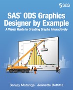
This example plots the Metropolitan Relative Weight (MRW), a measure of obesity, for a group of male and female participants. The example shows the association between obesity and mortality, while taking into account the effect of smoking.
The graph consists of a bar chart and a vertical axis table on the right Y axis.
Figure 6.2 Graph for this Example

Generate Bulk Graphs
The Auto Charts tool enables you to generate graphs in bulk from a list of variables that you specify and from graph types that you select. The following steps walk you through this process. Refer to Figure 6.1 when completing these steps.
1. Select Tools ► Auto Charts. The Auto Charts window is displayed.
2. In the top pane, complete these steps:
a. For Library, select SASHELP.
b. For Data Set, select HEART.
3. In the left pane, select the following check boxes:
SEX
MRW
AGEATDEATH
SMOKING_STATUS
The left and right panes of the Auto Charts window are resizable. If you cannot see the full variable names, you can drag the border of the left pane to widen it.
4. In the bottom portion of the left pane, select Grouped. The Select graph types group should look like the following image:

5. Click Generate Graphs. The right pane is populated with graph icons.
6. Take a moment to examine the graphs. Notice that all the icons are for single-cell graphs. You want to consider multi-cell graphs, so make a minor change to your selections, and generate another set of graphs.
7. In the right pane, click Delete All. This removes all of the icons from the pane.
8. In the left pane, select the Advanced Plots check box, and then click Generate Graphs. This time there are more results, and the icons include more advanced graphs such as classification panels and multi-cell graphs.
Customize Your Graph
After generating the graphs, you can choose one or more graphs as the starting point for customization.
Create Your Graph
For this example, use a simple bar chart. You start the graph by opening the graph’s icon.
1. In the right pane, select the icon for the horizontal bar chart with the title Metropolitan Relative Weight by Smoking Status and SEX, and then click Open. You can also double-click the icon.

The designer opens the bar chart in the work area as shown in Figure 6.3.
2. (Optional) If you right-click the bar chart, and select Assign Data, you see the following data assignments for the Category, Response, and Group variables:

You can change these data assignments as needed to create your graph.
Figure 6.3 Bar Chart
This simple graph contains all the information that you need except for the AGEATDEATH variable. For that, you add an axis table to the graph.
Add an Axis Table to the Graph
About the Axis Table
As described in the survival plot example in Chapter 5, an axis table is a basic plot that displays data values in textual form at specific locations along the vertical or horizontal axis. In this Auto Charts example, the axis table is placed in the same cell as the bar chart. Because it shares the same cell, the axis table must use the same library and data set as the bar chart.
For this axis table, specify a variable for Y to generate a vertical table. The variable identifies the locations along the Y axis. Specify a variable for Value. This variable determines which values are displayed in the axis table.
Create the Axis Table
First, create a vertical axis table that displays the age at death for male and female subjects. Assign data in the Assign Data dialog box. In addition, reposition the label for the axis table.
1. In the Elements pane, click the AxisTable icon, and drag and drop the icon onto the graph window.

The Assign Data dialog box is displayed. Library and Data Set are not available because the axis table must use the same data as the bar chart.
2. In the Assign Data dialog box, complete these steps:
a. For Y, select SMOKING_STATUS. This variable identifies the locations along the Y axis for the axis table. It aligns the axis table with the bars.
b. For Value, select AGEATDEATH. This variable determines which values are displayed in the axis table.
c. For Class, select SEX. This variable creates a separate column for each unique class value. It acts as a classification variable for the axis table.
d. For Group, select SEX. This variable groups the axis table. Each group value is represented by a different visual attribute.
e. For Position, select Right. This positions the table along the right Y axis.

f. Click OK. The axis table is added to the graph.

Next, move the axis table labels so that they appear above the axis table.
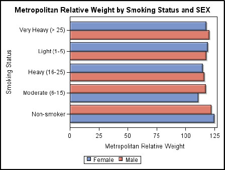
3. Right-click the axis table, and select Plot Properties. The Cell Properties dialog box is displayed with the Plots tab selected.
4. In the Cell Properties dialog box, complete these steps:
a. For Plot, select axistable if it is not already selected.
b. Click the Label tab, which is directly below Plot.
c. For Position, select Max. This moves the axis table’s labels to the maximum end of the axis.
d. Click OK.
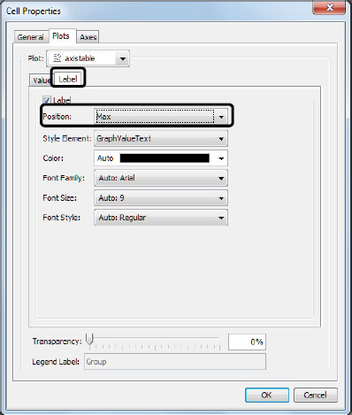
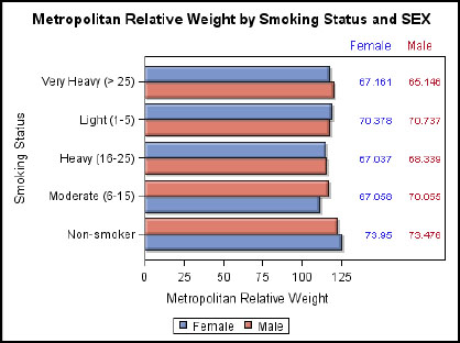
The graph is updated with your changes.
Figure 6.4 Bar Chart with Axis Table
Customize the Titles
The last step is to shorten the existing title and add a second title above the axis table.
1. Select the title. The text is highlighted.
2. Enter MRW by Smoking Status.
3. Select Insert ► Title.
4. Click outside of the placeholder title text to deselect it. Then, right-click the placeholder text, and select Title Properties.
5. In the Text Properties dialog box, complete these steps:
a. In Text Entry, enter Age at Death.
b. For Style Element, select GraphLabelText.
c. For Font Style, select Bold.
d. For Position, select Right. This positions the new title above the axis table.

e. Click OK.
The final graph is shown in Figure 6.2 and repeated here:
