
IN THIS CHAPTER
In the next four chapters, we will go over the system administration tasks you will have to know, whether you are managing a 1,000 seat network or a single system—your own.
Nearly everything you do in this chapter will be as Root/SuperUser. This is because you’re dealing with important system-related issues. As noted previously, when you are working with Root powers, you can do wonderful things quite easily. It is also just as easy to blow your system away. Take care.
Here you will learn about the different file systems SUSE Linux can use to format your drives and other storage devices.
You’ll learn about Logical Volume Management (LVM) and how to mount drives and add peripheral storage devices to your system, such as a USB key chain storage device.
Sometimes it’s hard to find a file or directory on a big system. Do you wonder if an application you heard about at the Linux User Group meeting is installed on your system? From the standard shell file-finders to the brand new Beagle graphical desktop search tool, you can find things relatively easily with the Linux tools you’ll learn about in this chapter.
We’ll also tell you about GNU Parted, the partitioning tool included with SUSE Linux.
This information is essential for Linux newbies, and old hands might pick up something new, too.
It’s always good to remember that in Unix/Linux, a file system is not just the hierarchy of files and directories accessible through the shell or a GUI file manager.
File systems include the disk format type and the metadata surrounding files and directories. Because everything in Linux is a file with properties, permissions, and other attributes, everything attached to the system (printers, mice, keyboards, files on network servers, remote machines, FTP servers, and so on) is part of the file system.
When we talk of choosing a file system, though, we’re talking about disk formats. The Linux kernel and SUSE Linux can work with many file systems. Table 18.1 shows the variety.
Table 18.1. Linux Compatibility with Various File Systems
Name | Description | Run Linux Natively | Read from Linux | Copy/Move Files |
|---|---|---|---|---|
ReiserFS | Default SUSE Linux file system. Journaled. | Y | Y | Y |
ext2 | Y | Y | Y | |
ext3 | ext2 with journal. | Y | Y | Y |
JFS | IBM Journaled file system. | Y | Y | Y |
XFS | Journaled file system originally for SGI IRIX, ported to Linux. | Y | Y | Y |
Minix | N | Y | Y | |
NFS | N | Y | Y | |
FAT12 | N | Y | Y | |
FAT16 | N | Y | Y | |
FAT32/vfat | Windows 9x file system. | N | Y | Y |
NTFS | N | Y | NTFS > Linux only. | |
HFS | N | Y | Y | |
ISO9660 | N | Y | Y | |
UDF | N | Y | Y |
All these file systems organize data on a disk in largely the same manner.
The differences between them, especially among the Unix/Linux file systems, are usually related to the speed of retrieval. Disks are organized (or formatted) in blocks. The first block of any disk is the boot sector, which contains a very short program (a few hundred bytes), which will load and start running the operating system.
In the case of a dual-boot system, a bootloading program, such as lilo or grub, will be stored there. All other blocks (sometimes called clusters or sectors) contain the operating system, all your application files, and all your data files that constitute your life.
In Unix and Linux, each block is 1024 bytes by default. A block contains several smaller bits of data:
A superblock, with redundant information about the complete file system.
More redundant file system descriptors, useful for reliability and disaster recovery. Also explains why it’s really hard to recover when you remove/delete a file in Unix/Linux. All the redundancy disappears, too.
A bitmap of the block.
A bitmap of the inode table (see the paragraph following this list for more on inodes).
Information from the inode table.
An inode contains all the information needed to identify a file—its attributes and permissions, its location(s)on the disk, its owner, timestamps—except the filename itself (which belongs to the directory).
There is one inode for every file. The inode table performs the same function as the DOS File Allocation Table (FAT). It keeps track of where files are located on the disk for easy retrieval.
ReiserFS version 3 is the default file system for SUSE Linux. Created from the ground up by Hans Reiser, it is safer and faster than the old default ext2 file system.
It is a journaling file system, meaning it has a file (a journal) that records changes to the file system. Should you have a system crash, a power surge, or some other mishap leading to an unexpected (that is, involuntary) shutdown, recovery will be less traumatic. ReiserFS was the first journaling file system included into the Linux kernel, and it has been supported since kernel version 2.4.1 in January 2001.
If you’ve ever had Microsoft Windows crash or freeze up, you’ll know the pain and agony associated with a nonjournaling file system.
Following the unexpected shutdown, Windows runs its ScanDisk program over your entire hard drive, checking for both bad disk sectors and reestablishing where every file snippet is physically located on the disk. Because broken links might occur, you may have orphaned clusters, a common problem that will result in a loss of data.
Although Linux is a much safer OS with far fewer software-related crashes, Linux users have not been entirely exempt from the involuntary shutdown. When this happens under the ext2 file system, the fsck program also scans the entire file system to make sure no data is lost in the crash. It could also take its time in processing the drive before you can log in.
The journal file makes it tremendously faster and easier to confirm that the disk is not damaged and that data is not lost. The journal knows what changes (saving new data, creating new files, deleting files, updating, and so on) were made to the disk since the last normal shutdown and tells the disk scanner where they are physically located on the disk. The scanner confirms that the location is not damaged and proceeds. This process does not guarantee that no data will be lost in this situation (the journal does not know what you typed since the last save before the crash), but it is in much better shape.
ReiserFS also manages blocks much differently than the Extended Filesystem (ext2, ext3), allowing many small files to share a block. This speeds retrieval and should display small files faster.
Its chief weakness is a problem only for people converting an existing ext2 or ext3 file system to ReiserFS. You must back up all your data and reformat the drive before installing ReiserFS. If you are installing SUSE Linux for the first time on your computer, this is nothing to worry about.
Note
The next generation of the ReiserFS, Reiser4, was released in early 2005. The file system, with financial help from the Defense Advanced Research Projects Agency (DARPA), has some advanced security features. These are outlined on the Namesys website: http://www.namesys.com/v4/v4.html#enh_security.
You can expect SUSE Linux to integrate Reiser4 in an upcoming release.
The ext2 file system was the standard and default throughout the early years of Linux kernel development. Hardly anyone used anything else until very recently. When ReiserFS first produced a journaling file system, Red Hat and others worked to bring journaling to this file system and ext3 was added to the kernel as of v2.4.16 in November 2001.
Ext3 and ext2 are nearly identical except for the journal file. If you are installing SUSE Linux over an existing ext2 file system, you might want to use ext3 instead of ReiserFS. The chief advantage of the ext3 file system is that it will automatically recognize files on ext2, and reformatting is not required.
IBM’s original Journaling File System (JFS) and the XFS file system from SGI (formerly Silicon Graphics, Inc.) are file systems that were designed for other Unix versions now ported to Linux. JFS was the file system of choice for AIX users. SGI created XFS to be the basis for its IRIX systems.
JFS introduced journaling to Linux, and has its own version of fsck to handle problem boots. XFS claims superior performance than either JFS or ReiserFS. Perhaps one of these will work for you.
Don’t fret endlessly over what file system to choose. All the file systems discussed here are excellent. It is a one-time decision, though. There is some pain involved with changing file systems after installation, especially when moving from ext2 or ext3 to ReiserFS. If you are connected to an existing AIX or IRIX network or you are transitioning from one of these enterprise Unixes, stick with the file system you have.
Otherwise, selecting the default ReiserFS is probably your best choice.
The first, and perhaps only, time you have to create a new file system on your Linux computer is when you first install the operating system. You learned the basics of how to do this in Chapter 3, “Installing SUSE Linux.”
If you add a second hard drive, or have set up a series of mount points that you decide to adjust in one way or another, you can go to the YaST Expert Partitioner tool to handle this task for you.
Note
Until GNU Parted came along, partitioning in Unix and Linux was handled by the standard fdisk shell utility. It works a little differently from its DOS namesake, but performs the same essential tasks: creating and modifying the partition table.
The main difference between fdisk and Parted/Expert Partitioner, aside from the GUI, is that fdisk does not preserve existing data. If you tell fdisk to make the root partition 10GB smaller and create a new partition where the old one was, fdisk will do exactly that. If there was data sitting on a block in the last 10GB, it will be overwritten.
Feel free to use fdisk from the shell if you prefer, knowing its limitations.
Expert Partitioner (EP) is a GUI version of GNU Parted integrated into YaST. If you have used either of the Windows third-party partitioning products—PartitionMagic or Partition Commander—you will find EP familiar.
It simplifies the partitioning process and can adjust the partition table without harming existing data. You should know what you’re doing before you begin, however. There is a reason it’s called Expert Partitioner.
Caution
Unless you are working with new or otherwise empty drives, Expert Partitioner can ruin some data or even your entire hard drive. This is a very rare occurrence, but if you’re making changes to your partition table in the middle of a thunderstorm, power surges can mess things up badly.
Always back up at least your most important files before using EP, even if you are not planning to touch that mount point! And use an Uninterruptible Power Supply (UPS) whenever you have important data of any kind on your computer. This is the minimum protection you need.
Now that all the warnings are out of the way, we can begin to work with EP. It is actually a very simple tool. To open it, go to YaST, System, Partitioner. YaST will repeat the warnings you’ve seen in this section and make you click Yes before opening the tool.
There you will see your current partition table laid out, as shown in Figure 18.1.
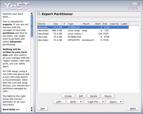
Figure 18.1. Expert Partitioner lets you resize existing partitions and create new ones. The initial screen displays your current partition table.
It’s a good idea to have a hard copy of all this information, so write it down in your notebook before making any changes.
In Figure 18.1, you can see that two physical hard drives are on this system: /dev/hda and /dev/sda. Each drive is 74.5GB after formatting. /dev/hda has two Linux partitions, Root (/) and Swap; /dev/sda has one Windows (NTFS) partition, seen here as /windows/C. The Start and End numbers are the block numbers, showing where on the disk each partition/mount point begins and ends.
Note
DOS/Windows (and practically all BIOS programs) supports only four primary partitions on a drive. Dual-boot systems have a particular problem with this setup. To get around this limitation, use the idea of turning one primary partition into an “extended partition” that allows you to create multiple “logical partitions,” making more efficient drives by making smaller sectors/blocks. There are few limitations on the number of logical partitions inside an extended partition.
You can install SUSE Linux into an extended partition; this is what YaST does by default. Linux file systems support up to 15 partitions/mount points.
Writing this information down is yet another safety valve in case of emergency, because you can reconstruct the table with the accurate start and end blocks if necessary.
At the bottom of the screen are eight action buttons that correspond to the task at hand. With EP, you can do the following:
Create a new partition from empty space on the disk.
Edit an existing drive or partition.
Delete an existing partition or drive (and all the data on it).
Resize a partition to make it larger or smaller.
Manage a logical volume (this is covered later in this chapter).
Create or manage a RAID volume structure (this is covered in Chapter 20, “Managing Data: Backup, Restoring, and Recovery”).
Encrypt a partition.
Reread or delete a partition table (under the Expert button).
The following sections walk you through these tasks.
Note
When you’re working with Expert Partitioner, you can do some experimentation without making changes to your system. Nothing you set up in the EP interface becomes final until you click Apply from the main window (refer to Figure 18.1).
Click Create to set up a new partition. Depending on your setup, you will be asked what disk to create the partition on and whether it is a primary or extended partition (see the preceding Note). EP then displays the Create Partition dialog box, shown in Figure 18.2.

Figure 18.2. The Create Partition dialog box lets you set all the necessary options for a new Linux partition.
Figure 18.2 shows the default settings for this dialog box. In addition to the ReiserFS, you can format the new partition as ext2, ext3, JFS, XFS, or as increased Swap. You can also create a FAT partition readable by Windows. The contents of the Options dialog box changes depending on the file system you choose.
A new partition can use only unformatted space on the physical drive. By default, EP will have this partition fill up the remaining free space, but you can choose to leave some space unformatted (and perhaps ready for another partition) by entering either a specific end cylinder or (as indicated) the size of the partition in megabytes (MB) or gigabytes (GB).
Tip
Check the Encrypt File System box to encrypt all new files created or moved into your new partition. See “Encrypting a Partition or Files” later in this chapter.
The Fstab Options button lets you set up Journaling mode (Ordered is the default), whether a user can mount this partition (No is the default), and whether to mount the partition automatically at startup (Yes is the default). You’ll learn more about the fstab file in the “Mounting a File System” section.
The last section is the mount point definition. The default here is /usr, but you can use the drop-down menu or type in a mount point as well.
When you select an existing partition and click Edit, the dialog box is nearly identical to Figure 18.2. All the options are editable except for the size parameters. You must use the Resize tool to change that.
Why would you edit a partition? If you want to use the Logical Volume Manager (LVM), at least one partition must have the type Ox8e or Ox83. You can set that in this dialog box. You may also want to change the fstab settings for a partition without editing the file by hand. Or you may want to change the mount point for one reason or another, especially with a nonroot partition.
There are only two reasons to delete a partition with EP: You’ve copied off all the data and want to recover the space for something else entirely, or you have a nonroot mount point that you don’t want to treat as a separate partition anymore.
The latter situation can occur when you define a mount point for /usr or /home to get a faster response from the disk, and the results are disappointing. In that case, move all the files back to the / partition before deleting the mount point.
To use EP to delete a partition, first unmount it with the umount command at the shell prompt. Open EP. Select the partition. Click Delete. You may get a warning, especially if you haven’t unmounted or if you accidentally selected the / partition. EP will then mark the partition for deletion. The delete action will not be final until you click Apply. After you do that, the partition will be gone, and the space will be available. See the section on umount later in this chapter.
This is the trickiest part of the EP process and is the special trick of GNU Parted. The standard Linux fdisk program creates, edits, and deletes partitions. But fdisk, like its DOS/Windows counterpart, is destructive when it performs its functions. fdisk will cheerfully create a new partition where some old data is lying around, but that data will be no more when it’s done.
Parted and EP will shrink an existing partition, taking care to preserve existing data and not overwrite it. You can then create new partitions on the empty space remaining.
To resize a partition, select the partition in EP and click Resize. The Resize dialog box (see Figure 18.3) appears.

Figure 18.3. Expert Partitioner shows you the amount of space being used by your partition. Use the slider or type in the size you want your new partition to be.
Use the slider, the spin box, or type in the size (in gigabytes) you want your new partition to be in the Unused Disk box. The second, bottom graphic will show what the disk will look like after the resizing takes place.
If you change your mind, click Do Not Resize to return the settings to where they were. If you are ready to proceed, click OK. The partition will be marked for resizing.
When you have confirmed your intention to resize the large partition, use Create as previously described to create the new partition(s) to fill the newly created space. After you’ve done that, click Apply to implement the new changes. You can turn back at any time before you click Apply.
If you run a business with your computer, you probably have some files that are more sensitive and valuable than others. You want to protect this information from prying eyes. Setting permissions and other access control tools is an important method of securing these files, but some things need even more security. This is especially true with data on laptops and removable hard drives.
SUSE Linux makes it possible, and relatively easy, to set up an area where files are encrypted within that space. You can set off an entire partition or create an encrypted file system within single files.
You have the option of creating encrypted partitions during the installation process, but you can also do this within EP.
Caution
Don’t use EP to encrypt a running file system! Adding encryption will destroy any data on a running partition. Always resize another partition and then create a new, encrypted partition using the preceding steps.
To create a single encrypted file to hold secure data, click Crypt File, Create Crypt File in the EP dialog box. Another dialog box (see Figure 18.4) appears.
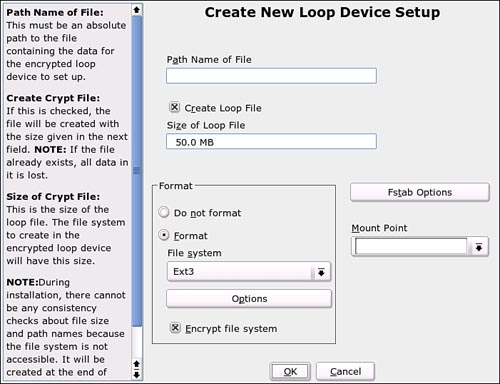
Figure 18.4. Use this dialog box to create a single file to hold secure data. When entering the pathname, do not point to an existing file unless you have it backed up.
Enter the path to the file to create along with its intended size. This is set to 50MB by default. Remember that this will be just one file, holding a spreadsheet with your balance sheets, for example. You want this file to be big enough to hold a growing file, but not so big that it encroaches on your capability to store other files. A good rule is to estimate how big that spreadsheet could get over the lifetime of your computer, and then double it.
SUSE recommends accepting the proposed settings for formatting and the file system type (that is, formatting for ext3). Specify the mount point. Decide whether the crypto file system should be mounted during boot in the fstab options. Click OK to mark this file for creation. EP will put this file at the end of the current partition. Your encrypted file will not be created until you click Apply at the end of the process.
To access an encrypted partition, you must use the mount command to make the partition visible. You will be asked to supply the password. See the section on the mount command later in the chapter.
Two Expert functions round out the EP tasks. If you suspect that the partition table is not showing up correctly in the EP window, click Reread Partition Table.
It’s not even close to being a common occurrence, but a bad label can get attached to a disk. If you’re having otherwise weird problems on your system, disposing of the label can be a last gasp. Delete Partition Table and Disk Label is the equivalent of waving the white flag and saying goodbye. Along with the bad label, everything else on that partition will disappear as well. Always back up before running this one.
A Linux system doesn’t really care what is attached to it at any given moment. Do you want to connect to a printer down the hall, a co-worker’s laptop in Australia, a backup mirror on the corporate server in Shanghai, or a floppy disk in your own machine? No problem—with the mount command and the right permissions, all these devices and file systems will appear on your system as if they were all just another part of your computer.
If you are the system administrator, you have near-absolute power over what file systems appear on your system, to whom, and when. In practice, this power is exercised through the use of the mount and umount commands, and through the /etc/fstab file governing file systems. In this section, you will learn about each of these tools.
The mount command loads a file system onto your computer and makes it visible. To mount a floppy disk, for example, insert the disk and then type the following (as SuperUser) at the shell prompt:
mount -t vfat /dev/fd0 /media/floppy
This is how the syntax breaks down (and you need all this to make it work):
Type (-t)—This flag and the next item identify the file system type for the platform to be mounted (in this case, the floppy is formatted for FAT32).
File system—Point to the device partition you are mounting. Floppy disks are, by default,
/dev/fd0. This information is set by and retrievable from/etc/fstab(see the section on/fstablater in the chapter).Mount Point—Where fstab actually looks for the files. In this case,
/media/floppy.
It is a good idea to have all your peripheral file systems (floppy drives, hard drives, USB and serial-port file storage devices, CD-ROM, DVD, and CD-RW drives) connected when you install SUSE Linux. Why? YaST can then identify all these devices and build your /etc/fstab file automatically.
Most of the time after you have mounted a hard drive or partition, you’ll keep it mounted. You’re always accessing it. Removable storage media are different; you’ll often pop one in, work on files (or copy/move them to your hard drive) and pop it out again. In Linux this is a little more complicated process.
After you have mounted a floppy as described in the last section, before you can put another floppy in the drive, you must unmount the drive. To do this, you must use the umount command (without an N):
umount /media/floppy
or
umount /dev/fd0
Before unmounting any file system, make sure that no processes are using files on that file system. You will get an error message if that’s the case.
The default file system mount behavior is set by the FileSystem TABle, or fstab. YaST sets this up during the initial installation. You can modify it directly in a text editor (as Root) or use Expert Partitioner’s partition editing tool. After you understand the structure of the file, it will be much easier to hand-edit etc/fstab, but EP’s fstab options page offers a friendlier interface if you are reluctant to hand-edit critical files.
Tip
You can view, but not edit, your fstab file in KdiskFree. This tool lets you see your current disk usage, device type, and mount point. You can mount unmounted file systems as well.
Here is a busy etc/fstab file, containing several drives and partitions, along with a CD-RW.
/dev/hda2  /            reiserfs  acl,user_xattr      1 1
/dev/sda1 /windows/C    ntfs       ro,users,gid=users,umask=0002,nls=utf8 0 0
/dev/hda1 swap          swap       pri=42             0 0
devpts   /dev/pts       devpts     mode=0620,gid=5    0 0
proc     /proc          proc       defaults           0 0
usbfs    /proc/bus/usb  usbfs      noauto             0 0
sysfs    /sys           sysfs      noauto             0 0
/dev/cdrecorder      /media/cdrecorder    subfs
fs=cdfss,ro,procuid,nosuid,nodev,exec,iocharset=utf8 0 0
/dev/fd0             /media/floppy        subfs
fs=floppyfss,procuid,nodev,nosuid,sync 0 0
Each line in the fstab file represents another device, file system, or hard drive. The order of items in each line are identical, with six fields altogether. You would guess (correctly) that all the items included in the mount syntax discussed earlier appear here. In order, they would be File system, Mount Point, and Type. The other items are various options that you did not set in the earlier simple example of the mount command.
The fourth field indicates the mount options for that file system, separated by commas. For example, the Windows drive, /dev/sda1, mounts as read-only (ro) and all users can mount the drive. If the user flag is not set, only Root can mount the file system. /dev/cdrecorder includes the exec option, which allows you to run binaries from the CD drive. The / (Root) partition uses an Access Control List (ACL) to determine whether binaries can be executed. This means permissions are set at a lower, more fine-grained level than just allowing anyone with access to the partition to execute programs.
The other options listed here are generally specific to that file system. To see all the options that can be used here, see the mount and fstab man pages.
The last two fields (in the example, all are marked 0 0 except for /, which is 1 1) are digits that other programs use. The fifth field tells dump, a venerable Unix backup program, whether to back up the file system when it is run: 1=Yes, 0=No.
The last field tells the file system repair tool fsck how to interact with each file system: 0=Never, 1=Run at a designated time, 2=Run periodically, but less often than the 1s.
You should not have to edit /etc/fstab more than once, but if you have problems with the OS not seeing a file system (CD won’t run, can’t copy files from a floppy or Zip disk, for example), this is usually the place to start troubleshooting.
The dilemma in partitioning has always been how large to make each partition (also known as a volume). Too often, you just accept a default, or make a wild guess about how much space you’ll need for the data you plan to put on your partition. One day, you’ll find yourself painfully short of space on one volume, while having a ton of room on another. Wouldn’t it be great to have some space that you could allocate on-the-fly, even while a partition was already mounted? Logical Volume Management is a relatively new technology that allows you to use disk space from multiple drives in a single logical volume.
The LVM module in YaST is located under the System page. When you open it the first time, it asks you to create a Volume group. It’s best to accept the default and create a System group, but allocate as much space as you want for your Volume group.
A Volume group identifies the Physical Volumes (PVs) on your system. These are the building blocks for your Logical Volumes (LVs). To create a new LV, click Add under the logical volume pane. You will need to specify a size and a file system (like ReiserFS). Click Finish to mount the new volumes.
When it’s time to resize your LVs, return to this module. Select the volume you want to shrink and click Edit. Make this volume smaller, and then select the volume you want to expand. Edit it.
LVM works on any Linux file system and can also be used to create more swap space.
With this in mind, let’s discuss how you find files within your file system.
From time to time, you will need to locate a particular file in your file system. With SUSE Linux, you have a variety of tools available to do this. We’ll discuss how to use the find, locate, which, and whereis commands, as well as several graphical utilities to track down files.
The findutility does just what its name implies. It’s used to find files in your computer’s file system. The syntax for using find is as follows:
find path search_pattern
One of the advantages of find is that you can use a variety of search patterns. You can search for a filename, for a specific file type, for files of a particular size, for files that were modified at a certain time, and for files owned by a particular user or group.
These search patterns are created using the following command-line options:
-name“file_name”—This option allows you to search for a filename. You can use a specific filename or you can use a wildcard pattern.-size + or –size—This option allows you to search for files that are smaller than or larger than the specified size.-typetype—This option allows you to specify whether you are looking for directories (d), files (f), or symbolic links (l).-ctime + or –days—This option allows you to search for files that were modified more or less than a specified number of days ago.-groupgroup_name—This option allows you to search for files that are owned by a specific group.-
useruser_name—This option allows you to search for files that are owned by a specific user.
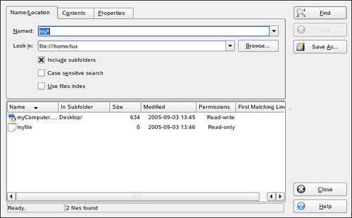
For example, suppose you wanted to find a file named myfiles that you think resides in the /home/tux directory on your system. You could enter find /home/tux -name “myfiles” at the shell prompt. The find utility will then search the /home/tux path for any file named myfiles, as shown in Figure 18.5.

The find utility, by default, searches all subdirectories beneath the path specified. In the preceding example, you could also enter find / -name “myfiles” at the shell prompt and it would find the /home/tux/myfiles file (although it will take much longer). For more information about how to use find, enter man find at the shell prompt.
In addition to find, you can also use the locate utility to search for files. Let’s look at this utility next.
The find utility works great for locating files in the file system. However, it has one drawback. It finds files by searching through each and every directory beneath the path specified in the command line. This process can be quite slow. For example, if you were to use find to create a search that searched for a specific file from the top of the file system, it may take 10 to 15 minutes (possibly longer) to complete.
As an alternative, you can use the locate utility to search for files. The locate utility operates using an entirely different search mechanism. Instead of searching through directories, it looks for the specified file within its own database of files that are stored in the system.
The locate utility is part of the findutils-locate package. Before you can use locate, you must use YaST to install this package on your system, as shown in Figure 18.6.

After these packages are installed, a database is created in /var/lib called locatedb. A listing of files in your file system is stored in this database. This database is automatically updated every day. If necessary, you can also manually update it by running the updatedb utility from the shell prompt.
With the database updated, you can use the locate utility to search for files within it. The syntax for using locate is relatively simple. You simply run locate and specify the name of the file you want to search for, as shown next:
locate file_name
For example, if you wanted to search for the myfiles file, you would enter locate myfiles, as shown in Figure 18.7.

As with find, you can view the man page for the locate utility to learn more.
In addition to find and locate, you can also use the which command to search for files. Let’s review this command next.
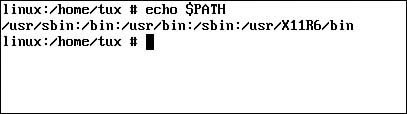
The whichutility is a handy command for finding the executable files used by system commands. The which utility searches for files in a manner similar to the find utility. However, which searches for files only in the directories contained in the PATH variable.
At this point, you’ve probably noticed that you can run system commands, such as which, locate, find, cp, rm, and cd, regardless of what your current directory in the file system is. That’s because the executable files for these commands reside in directories that are included in the PATH variable. You can see a listing of these directories by entering echo $PATH at the shell prompt, as shown in Figure 18.8.
The which utility is used to generate a search that is limited to the directories in the PATH variable. For example, if you wanted to find out where the cp executable resides, you would enter the following:
which cp
The which utility then returns the path where cp is located, as shown in Figure 18.9.

When working with system commands, you can also use the whereis utility. Let’s explore this command next.
Like which, the whereis utility is used to find the location in the file system where system commands reside. However, it can return much more information about the file than which can. It not only returns the location of the file, it also returns the location of the man page file and of the source code file (if it exists).
The syntax for using whereis is relatively straightforward. Enter
whereis command
For example, if you wanted to get information about the rm command, you would enter the following:
whereis rm
The whereis utility then returns the relevant data, as shown in Figure 18.10.

If you want to limit the output provided by whereis, you can use the following syntax:
whereis option command
The options you can use include the following:
-b: Returns only the location of the command in the file system.-m: Returns only the name and location of the command’s associated man page files.-s: Returns only the name and location of the command’s associated source code file.
In addition to these command-line utilities, SUSE Linux also includes graphical utilities that can be used to search for files. Let’s look at these next.
The first utility we will explore is kfind, which is a graphical version of find that runs within the KDE shell. To use KFind, select K Menu, Find Files/Folders. The screen in Figure 18.11 is displayed.
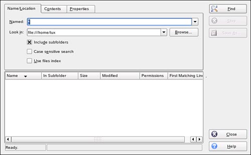
Within this interface, you can configure and execute complex search operations. To do this, complete the following:
In the Named field, enter the name of the file you want to search for. You can use wildcard characters such as * and ? to expand your search results.
In the Look In field, enter the path in which
kfindshould begin its search.If you want
kfindto search for the specified file in subdirectories within the specified path, mark Include Subfolders.Select Find. The results of your search are displayed in the field below the search criteria, as shown in Figure 18.12.
In addition to kfind, you can also use a new, more advanced graphical search tool on SUSE Linux: Beagle.
Beagle is a search tool that can be used to find different types of information from a variety of data sources associated with your user account. Beagle can search your personal documents, text files (including source code), email, browser history, instant messages, web pages on the Internet, man pages, help files, and media files.
To use Beagle, you must first install the beagle package on your system using YaST, as shown in Figure 18.13.

Be warned; the Beagle package has a number of dependencies that will need to be installed along with it. When you select Accept in YaST, a screen will be displayed listing the additional packages that must be modified or installed to support Beagle, as shown in Figure 18.14.

After you have Beagle installed, the next thing you need to do is start the daemon. It’s important that you understand that the Beagle daemon operates in a different manner from other system daemons you may be familiar with. Most other daemons run as either your root user or another specialized user account.
The Beagle daemon, on the other hand, is run from within your individual user account. This is because Beagle searches for data that exists within your own user “space.” To start the Beagle daemon, open a terminal session and enter beagled at the shell prompt. The daemon will run in the background and begin automatically indexing content available to your user account.
If you want to customize how the daemon behaves, you can run the Beagle configuration utility by entering beagle-settings from the shell prompt. When you do, the screen shown in Figure 18.15 is displayed.
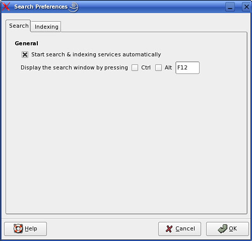
Under the Search tab, you can configure whether beagled automatically starts searches and indexing as well as the hotkey sequence required to open the search window. You can configure what beagled will index by selecting the Indexing tab, shown in Figure 18.16.

Under this tab, you can configure specific directories that should be indexed and other directories that should not be indexed. By default, all subdirectories of the directories specified are included. As the daemon is running, you can see the content it has indexed by entering beagle-index-info at the shell prompt.
Beagle will conduct its searching and indexing operations in the background and run with a low priority so that it doesn’t take up excessive amounts of CPU time or hard disk bandwidth. In this mode, the indexing operation could take many hours to complete. However, you can force beagled to run at a higher priority and complete the index process much faster. This is done by stopping the daemon, entering export BEAGLE_EXERCISE_THE_DOG=1 at the shell prompt, and then restarting the daemon.
After your indexing is complete, you can use the Bleeding Edge Search Tool (BEST) to search for data. At the shell prompt, enter best –show-window. The screen in Figure 18.17 is displayed.
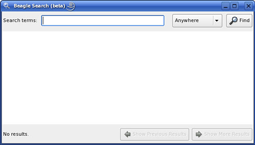
In the Search Terms field, you can enter the text you want to search for. In the drop-down list, select the data source you want to search, and then select Find.
You can also use a web browser to compose and execute searches. The Beagle daemon includes a small web server application that is enabled by default on port 8888. To access the beagled daemon through a browser window, navigate to http://localhost:8888/beagle/search.aspx.
With this in mind, let’s now discuss some more advanced tasks you can perform with your Linux file system.
For some people, reading books and going to lectures or discussions are the best way to learn new things. For others, playing around on a system is the way to go. If you want to see for yourself how things work in different file systems, try creating a file system using the loopback file system—a special file system that lets you accomplish this interesting and useful feat. You can use the file system you create to experiment with and practice almost all the shell commands found in this chapter with no fear of damaging your system.
Tip
To do this on a larger scale, you can install a basic SUSE Linux system into the Xen virtual machine. Pick a file system, don’t install the graphical end, and you have another playground apart from your working system. See the Xen section of Chapter 11, “Going Cross-Platform,” for details.
People who run Linux tend to be a tinkerer’s lot. They like to try new things and are not afraid of getting under the hood and plumbing the depths of their computers to see what exactly is going on. Although many Linux users have multiple machines (and parts of machines) cluttering up the house, most people have just one computer with a single hard drive to play with. If you then have data on that computer that is really important, you don’t want to blow away your operating system on a regular basis after an experiment goes awry. This is perhaps the reason the loopback file system was born. With this handy tool, you can create an image file containing the file system of your choice, and mount it—leaving your “real” file system alone and safe.
You could do this exercise on a floppy or other removable drive, but if you want ample room to play in, working off a hard drive is a better way.
Use the dd command to create a file with a block size of 1,024 bytes (a megabyte) and create a file that is 10MB in size. You should have enough free space on your drive to accommodate a file that size, of course. You need 10,000 blocks of 1KB (1,024 bits) in this 10MB file, so here’s what you type:
Dd if=/dev/zero of=/tmp/test-img bs=1024 count=10000
The shell responds with
10000+0 records in
10000+0 records out
Now we need to make the system think the file is a block device instead of an ASCII file, so we use losetup, a utility that associates loop devices with regular files or block devices. You will use the loopback device /dev/loop0. losetup /dev/loop0 /tmp/test-img.
Then format the file with an ext3 file system:
mkfs -t ext3 -q /tmp/test-img
If prompted that test.img is not a block device, enter y to proceed anyway.
Your test file system is ready to go, except that you can’t do much with it until it is mounted on your system. Let’s start with a mount point, then.
mkdir /mnt/image
Now we can mount it:
mount –o loop /tmp/test.img /mnt/image
After mounting the file system, look at it with the df command:
df –h /mnt/image
And get this response:
Filesystem        Size    Used    Avail    Use%    Mounted on
/tmp/test-img     10M     1.1M    9M       2%      /mnt/image
To unmount the image:
umount /mnt/image
You can even back up the image, in case something happens while you’re playing:
cp /tmp/test-img test-img.bak
When you’ve confirmed that you have a mounted image file, you can create directories, copy files to it, delete files, attempt to recover them, and, generally speaking, do anything you want with this file system. It’s a playpen where you can learn valuable lessons with no risk. If you somehow irreparably damage the file system on the image, unmount it, delete it, and start over, perhaps with that backup you just made. So have fun!
Let’s now discuss how to mount a read-only partition on a running system.
From time to time, you may need to mount a partition in your file system in such a manner that you can view the data that it contains but not be able to make changes to it. This can be accomplished by mounting the partition in read-only mode. You can do this in two ways. The first is with the mount command. At the shell prompt, enter
mount -r device mount_point
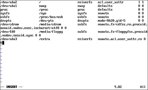
For example, if you had a partition at /dev/sda3 and you wanted to mount it at the /extra directory, you would enter the following:
mount -r /dev/sda3 /extra
This is shown in Figure 18.18.
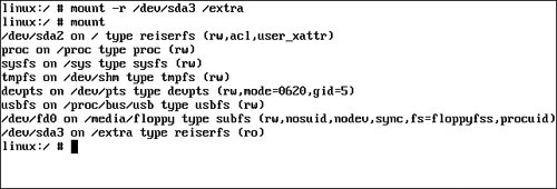
In Figure 18.18, you can see that the /dev/sda3 partition is mounted in the /extra directory. Notice that when the mount command is subsequently issued without arguments, the mounting for /dev/sda3 is shown with a (ro) designation, indicating that the partition is mounted read-only.
In addition to using mount, you can automatically mount the partition read-only using your fstab file. Simply add ro to the mount options field, as shown in Figure 18.19.
With this in mind, let’s now look at mounting an image file as a floppy disk device.
Earlier in this chapter, you learned how to mount floppy disks on your SUSE Linux system. Using the loopback filesystem, you can also mount an image file as a floppy disk. This is done by completing the following:
Open a terminal session.
Switch to your root user.
Create the image file by entering
dd if=/dev/zero of=floppy.img bs=512 count=2880at the shell prompt.At the shell prompt, enter
losetup /dev/loop0 floppy.img.Format the file using the MSDOS file system by entering
mkdosfs /dev/loop0at the shell prompt.Mount the image file as a floppy by entering
mount -t msdos /dev/loop0 /media/floppy.
This process is shown in Figure 18.20.

Before ending this chapter, we need to discuss one more topic: working with character and block devices. Let’s look at this next.
As you’ve probably noticed as we’ve gone through this chapter, every device in your SUSE Linux system is represented as a file in the /dev directory. Your hard disk drive is represented as a file, such as hda (IDE) or sda (SCSI). Your floppy disk drive is represented as a file, such as fd0. Even your CD-ROM drive is represented by the cdrom file, which is actually a symbolic link to another file, such as hdb or hdc. These files allow your hardware devices to function as one of the following device types:
Character devices—Character devices transfer data in a serial fashion, one piece of information at a time. Modems, keyboards, mice, and terminals are examples of character devices.
Block devices—Block devices are those that, unlike a character device, provide a degree of random access to the data they contain. Hard disk drives, floppy disk drives, and CD/DVD drives are examples of block devices.
Every device in your system needs a driver for the Linux kernel to be able to interface with it. For example, your IDE hard disk drive needs a driver; all SCSI devices in your system need a device driver as well. An important point to remember is that multiple devices of the same type can be serviced by the same kernel driver. For example, if you had three SCSI hard drives in your system, a single instance of the SCSI kernel driver can manage the three physically separate devices.
The Linux kernel keeps track of these different devices using major and minor device numbers. These numbers are assigned to each device’s associated file in /dev. The major number indicates the type of device associated with the file. For example, consider the files displayed in Figure 18.21.

In Figure 18.21, the ls -l command has been used to display the various IDE device files in /dev, denoted as hda. Notice in the middle of each line in the output of ls that two numbers are displayed. The first number is the major number. All IDE devices have a major number of 3. (SCSI devices have a major number of 8.) The major number identifies which device driver the kernel should use to interface with the particular device.
In Figure 18.21, you will also see a second number listed in the middle of each line of the output of ls. This is the minor number. For example, device file hda has a major number of 3 and a minor number of 0. The minor number identifies the specific node of the device. In Figure 18.21, you can see that device hda1 (the first partition on the master IDE hard drive on the primary IDE channel) has a major number of 3 and a minor number of 1.
In addition, the output of ls, shown in Figure 18.21, indicates the type of device represented by each file. This is indicated by the first character of each line. Notice that each hda line in Figure 18.21 begins with a b. This indicates that the IDE hard disk drives are block devices. By way of comparison, refer to Figure 18.22.

The tty devices shown in 18.22 are serial devices. Accordingly, they have a c as the first character in each line of the output of ls, indicating that these files represent character devices.
You can create your own character or block device files. This is done with the mknod utility. The syntax of mknod is as follows:
mknod file_name device_type major_number minor_number
For example, you could create a new character device named echo with a major number of 33 and a minor number of 0 by entering the following at the shell prompt:
mknod /dev/echo c 33 0
Major number 33 (character) is reserved for serial cards. You can view a complete list of major numbers and the type of devices they are associated with by viewing the /usr/src/linux-kernel_version/Documentation/devices.txt file on your SUSE Linux system.
http://www.tldp.org/HOWTO/Filesystems-HOWTO.html—Always the place to begin. The file systems HOWTO.
http://en.wikipedia.org/wiki/Filesystem—Wikipedia on how file systems work in various operating systems.
http://en.wikipedia.org/wiki/Comparison_of_file_systems—Helpful chart on differences between file systems, with links to the Wikipedia articles on each file system.
http://www.namesys.com—The group in charge of ReiserFS.
http://batleth.sapienti-sat.org/projects/FAQs/ext3-faq.html—The Linux ext3 FAQ list. Differences between ext2 and ext3, as well as troubleshooting problems.
http://oss.sgi.com/projects/xfs—The XFS for Linux site.
http://www-106.ibm.com/developerworks/linux/library/l-fs9.html—An IBM DeveloperWorks article on XFS.
http://www-106.ibm.com/developerworks/edu/os-dw-linuxjfs-i.html—A JFS tutorial; free registration with DeveloperWorks required.
http://sources.redhat.com/lvm2—The Logical Volume Manager home page.
http://www.tldp.org/HOWTO/LVM-HOWTO—The LVM HOWTO page. Should have information on LVM2 by now.
http://usalug.org/phpBB2/viewtopic.php?p=33142—Tuning up IDE hard drives with hdparm. A useful tutorial.
http://www.gnu.org/software/parted—The GNU Parted home page.
http://www.freeos.com/articles/3921—A basic introduction to the Logical Volume Manager. Includes command-line instructions for building logical volumes.