
We’ve covered most of the basics you need to know about how formulas and references work. In the following sections, we’ll dig deeper, covering how to use defined names, intersections, structured references, and three-dimensional (3-D) formulas.
If you find yourself repeatedly typing cryptic cell addresses, such as Sheet3!A1:AJ51, into formulas, we’ll show you a better approach. You can assign a short, memorable name to any cell or range and then use that name instead of the cryptogram in formulas. Naming cells has no effect on either their displayed values or their underlying values—you are just assigning "nicknames" you can use when creating formulas.
After you define names in a worksheet, those names become available to any other worksheets in the workbook. A name defining a cell range in Sheet6, for example, is available for use in formulas in Sheet1, Sheet2, and so on, in the workbook. As a result, each workbook contains its own set of names. You can also define worksheet-level names that are available only on the worksheet in which they are defined.
Note
For more information about worksheet-level names, see "Workbook-Wide vs. Worksheet-Only Names".
When you use the name of a cell or a range in a formula, the result is the same as if you typed the cell or range address. For example, suppose you typed the formula =A1+A2 in cell A3. If you assigned the name Mark to cell A1 and the name Vicki to cell A2, the formula =Mark+Vicki has the same result and is easier to read.
The easiest way to define a name follows:
Select a cell.
Click the Name box on the left end of the formula bar, as shown in Figure 13-10.
Type TestName, and then press Enter.

Keep the following basics in mind when using names in formulas:
The Name box usually displays the address of the selected cell. If you have named the selected cell or range, the name takes precedence over the address, and Excel displays it in the Name box.
When you define a name for a range of cells, the range name does not appear in the Name box unless you select the same range.
When you click the Name box and select a name, the cell selection switches to the named cells.
If you type a name in the Name box that you have already defined, Excel switches the selection instead of redefining the name.
When you define a name, the stored definition is an absolute cell reference that includes the worksheet name. For example, when you define the name TestName for cell A3 in Sheet1, the actual name definition is recorded as Sheet1!$A$3.
Note
For more information about absolute references, see "Understanding Relative, Absolute, and Mixed References".
Instead of coming up with new names for cells and ranges, you can simply use existing text labels to create names. Click the Define Name button on the Formulas tab on the Ribbon to display the New Name dialog box shown in Figure 13-11. In this example, we selected cells B4:E4 before clicking the Define Name button, and Excel correctly surmised that the label Region 1 was the most likely name candidate for that range. If you are happy using the adjacent label as a name, just press Enter to define the name, or you can first add a note in the Comment box if you want to provide some helpful documentation.

Figure 13-11. When you click Define Name on the Formulas tab, Excel suggests any label in an adjacent cell in the same row or column as a name.
You can, of course, define a name without first selecting a cell or range on the worksheet. For example, in the New Name dialog box, type Test2 in the Name text box, and then type =D20 in the Refers To text box. Click OK to add the name, which also closes the New Name dialog box. To see a list of the names you have defined, click the Name Manager button on the Formulas tab. The Name Manager dialog box appears, as shown in Figure 13-12.


Figure 13-12. The Name Manager dialog box provides central control over all the names in a workbook.
The Name Manager dialog box lists all the names along with their values and locations. You’ll see that the Refers To text box shows the definition of the name we just added, =Sheet1!D20. Excel adds the worksheet reference for you, but note that the cell reference stays relative, just as you typed it, while the Region_1 definition created by Excel uses absolute references (indicated by the dollar signs in the Refers To definition). Also note that if you do not enter an equal sign preceding the reference, Excel interprets the definition as text. For example, if you typed D20 instead of =D20, the Refers To text box would display the text constant ="D20" as the definition of the name Test2.
When working with tables created using the new table features in Excel, some names are created automatically, and others are implied. If this sounds intriguing, see "Using Structured References".
Although it is possible to edit name references directly using the Refers To text box in the Name Manager dialog box, it is preferable to click the Edit button at the top of the dialog box. Doing so opens the Edit Name dialog box, which is otherwise the same as the New Name dialog box shown in Figure 13-11. Although you can edit name references directly in the Name Manager dialog box, the Edit Name dialog box offers additional opportunities to change the name and to add a comment.
In the Edit Name dialog box, you can change cell references in the Refers To text box by typing or by directly selecting cells on the worksheet. When you click OK in the Edit Name dialog box, the Name Manager dialog box reappears, displaying the updated name definition. Clicking the New button in the Name Manager dialog box predictably displays the New Name dialog box; clicking the Delete button removes all selected names from the list in the Name Manager dialog box. Keep in mind that when you delete a name, any formula in the worksheet referring to that name returns the error value #NAME?.
Names in Excel usually function on a workbook-wide basis. That is, a name you define on any worksheet is available for use in formulas on any other worksheet. But you can also create names whose scope is limited to the worksheet level—that is, names that are available only on the worksheet in which you define them. You might want to do this if, for example, you have a number of worksheets doing similar jobs in the same workbook and you want to use the same names to accomplish similar tasks on each worksheet. To define a worksheet-only name, click the Scope drop-down list in the New Name dialog box, and select the name of the worksheet to which you want to limit the scope of the name.
For example, to define TestSheetName as a worksheet-only name in Sheet1, select the range you want, click the Define Name button on the Formulas tab, type TestSheetName in the Name text box, and then select Sheet1 from the Scope drop-down list, as shown in Figure 13-13.

Figure 13-13. Use the Scope drop-down list to specify a worksheet to which you want to restrict a name’s usage.
The following are some additional facts to keep in mind when working with worksheet-only and workbook-level names:
Worksheet-only names do not appear in the Name box on the formula bar in worksheets other than the one in which you define them.
When you select a cell or range to which you have assigned a worksheet-only name, the name appears in the Name box on the formula bar, but you have no way of knowing its scope. You can consider adding clues for your own benefit, such as including the word Sheet as part of all worksheet-only names when you define them.
If a worksheet contains a duplicate workbook-level and worksheet-only name, the worksheet-level name takes precedence over the book-level name on the worksheet where it lives, rendering the workbook-level version of the name useless on that worksheet.
You can use a worksheet-only name in formulas on other worksheets by adding the name of the worksheet followed by an exclamation point (no spaces) preceding the name in the formula. For example, you could type the formula =Sheet1!TestSheetName in a cell on Sheet3.
You can’t change the scope of an existing name.
You can click the Create From Selection button on the Formulas tab on the Ribbon to name several adjacent cells or ranges at once, using row labels, column labels, or both. When you choose this command, Excel displays the Create Names From Selection dialog box shown in Figure 13-14.

Figure 13-14. Use the Create Names From Selection dialog box to name several cells or ranges at once using labels.
Selecting Cells While a Dialog Box Is Open
The Refers To text boxes in the New Name and Name Manager dialog boxes (and many other text boxes in other dialog boxes) contain a collapse dialog button, which indicates that this is a text box from which you can navigate and select cells on the worksheet. For example, after you click the Refers To text box, you can click outside the dialog box to select any other worksheet tab, drag scroll bars, switch workbooks, or make another workbook active. In addition, if you click the collapse dialog button, sure enough, the dialog box collapses, letting you see more of the worksheet:

You can drag the collapsed dialog box around the screen using its title bar. When you finish, click the collapse dialog button again, and the dialog box returns to its original size.
Excel assumes that labels included in the selection are the names for each range. For example, Figure 13-14 shows that with A3:E7 selected, the Top Row and Left Column options in the Create Names dialog box are automatically selected, creating a set of names for each quarter and each product. Note that when using Create From Selection, you need to select the labels as well as the data. When you click the Name Manager button, you’ll see the names you just created listed in the dialog box.
You can create names that are defined by constants and formulas instead of by cell references. You can use absolute and relative references, numbers, text, formulas, and functions as name definitions. For example, if you often use the value 8.3% to calculate sales tax, you can click the Define Name button, type the name Tax in the Name box, and then type 8.3% (or .083) in the Refers To text box. Then you can use the name Tax in a formula, such as =Price+(Price*Tax), to calculate the cost of items with 8.3 percent sales tax. Note that named constants and formulas do not appear in the Name box on the formula bar, but they do appear in the Name Manager dialog box.
You can also enter a formula in the Refers To text box. For example, you might define the name Price with a formula, such as =Sheet1!A1*190%. If you define this named formula while cell B1 is selected, you can then type =Price in cell B1, and the defined formula takes care of the calculation for you. Because the reference in the named formula is relative, you can then type =Price in any cell in your workbook to calculate a price using the value in the cell directly to the left. If you type a formula in the Refers To text box that refers to a cell or range in a worksheet, Excel updates the formula whenever the value in the cell changes.
When you are creating a named formula that contains relative references, such as =Sheet1!B22+1.2%, Excel interprets the position of the cells referenced in the Refers To text box as relative to the cell that is active when you define the name. Later, when you use such a name in a formula, the named formula uses whatever cell corresponds to the relative reference. For example, if cell B21 was the active cell when you defined the name Fees as =Sheet1!B22+1.2%, the name Fees always refers to the cell one row below the cell in which the formula is currently located.
You can create three-dimensional names, which use 3-D references as their definitions. For example, suppose you have a 13-worksheet workbook containing one identical worksheet for each month plus one summary sheet. You can define a 3-D name that you can use to summarize totals from each monthly worksheet. To do so, follow these steps:
Select cell B5 in Sheet1 (the summary sheet).
Click the Define Name button.
Type Three_D (or any name you choose) in the Name box, and type =Sheet2:Sheet13!B5 in the Refers To text box.
Press Enter (or click OK).
Now you can use the name Three_D in formulas that contain any of the following functions: SUM, AVERAGE, AVERAGEA, COUNT, COUNTA, MIN, MINA, MAX, MAXA, PRODUCT, STDEV, STDEVA, STDEVP, STDEVPA, VAR, VARA, VARP, and VARPA. For example, the formula =MAX(Three_D) returns the largest value in the three-dimensional range named Three_D. Because you used relative references in step 3, the definition of the range Three_D changes as you select different cells in the worksheet. For example, if you select cell C3 and display the Name Manager dialog box, =Sheet2:Sheet13!C3 appears in the Refers To text box.
Note
For more information on three-dimensional references, see "Creating Three-Dimensional Formulas".
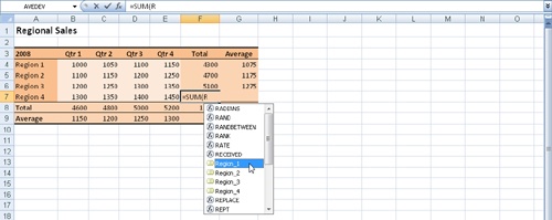
After you define one or more names in your worksheet, you can insert those names in formulas using one of several methods. First, if you know at least the first letter of the name you want to use, you can simply start typing to display the Formula AutoComplete drop-down list containing all the names beginning with that letter (along with any built-in functions that begin with that letter), as shown in Figure 13-15. To enter one of the names in your formula, double-click it.
Note
For more information, see "Using Formula AutoComplete".
You can also find a list of all the names relevant to the current worksheet when you click the Use In Formula button on the Formulas tab on the Ribbon, which you can click while in the process of entering a formula, as shown in Figure 13-16.

Figure 13-16. Click the Use In Formula button, and select a name to enter it into the selected cell.
Clicking the Paste Names command at the bottom of the Use In Formula menu displays the Paste Name dialog box shown on the left in Figure 13-17 when you are editing a formula. If you click the command when you are not in Edit mode, a different version of the dialog box appears, as shown on the right in Figure 13-17. The difference is the Paste List button, which we’ll discuss in the next section.
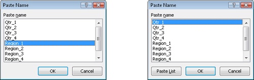
In large worksheet models, it’s easy to accumulate a long list of defined names. To keep a record of all the names used, you can paste a list of defined names in your worksheet by clicking Paste List in the Paste Name dialog box, as shown in Figure 13-18. Excel pastes the list in your worksheet beginning at the active cell. Worksheet-only names appear in the list only when you click Paste List on the worksheet where they live. Paste List is really the only useful feature in the Paste Name dialog box, given the superior methods of using names described in the previous section.

You can replace cell references with their corresponding names all at once using the Apply Names command, which you access by clicking the arrow next to the Define Name button on the Formulas tab on the Ribbon. When you do so, Excel locates all cell and range references for which you have defined names and replaces them with the appropriate name. If you select a single cell before you click the Apply Names command, Excel applies names throughout the active worksheet; if you select a range of cells first, Excel applies names to only the selected cells.
Figure 13-19 shows the Apply Names dialog box, which lists all the cell and range names you have defined. Select each name you want to apply, and then click OK.
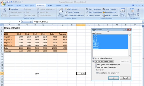
Figure 13-19. Use the Apply Names dialog box to substitute names for cell and range references in your formulas. Click Options to display all the options shown here.
Excel ordinarily does not apply the column or row name if either is superfluous. For example, Figure 13-19 shows a worksheet after we applied names using the default options in the Apply Names dialog box. Cell I17 is selected, and the formula bar shows it contains the formula =Region_2 Qtr_3, which before applying names contained the formula =D5. Because cell I17 isn’t in the same row or column as any of the defined ranges, both the row and column names are included in the new formula. Cell D17 contained the same formula, =D5. But because D17 is in the same column as the referenced cell, only the row name is needed thanks to implicit intersection, resulting in the formula =Region_2.
If you prefer to see both the column and row names even when they are not necessary, clear the Omit Column Name If Same Column check box and the Omit Row Name If Same Row check box.
The Name Order options control the order in which row and column components appear. For example, if we applied names using the Column Row option, the formula in cell I17 in Figure 13-19 would become =Qtr_3 Region_2.
Note
For more information about implicit intersection, see "Getting Explicit About Intersections" below.
Select the Ignore Relative/Absolute check box to replace references with names regardless of the reference type. In general, leave this check box selected. Most name definitions use absolute references (the default when you define and create names), and most formulas use relative references (the default when you paste cell and range references in the formula bar). If you clear this check box, absolute, relative, and mixed references are replaced with name definitions only if the definitions use the same reference style.
The Use Row And Column Names check box is necessary if you want to apply names in intersection cases, as we have shown in the examples. If you define names for individual cells, however, you can clear the Use Row And Column Names check box to apply names to only specific cell references in formulas.
When you click the Find & Select button on the Home tab and click Go To (or press F5), any names you have defined appear in the Go To list, as shown in Figure 13-20. Select a name, and click OK to jump to the range to which the name refers. Note that names defined with constants or formulas do not appear in the Go To dialog box.

In the worksheet in Figure 13-19, if you type the formula =Qtr_l*4 in cell I4, Excel assumes you want to use only one value in the Qtr_1 range B4:B7—the one in the same row as the formula that contains the reference. This is called implicit intersection. Because the formula is in row 4, Excel uses the value in cell B4. If you type the same formula in cells I5, I6, and I7, each cell in that range contains the formula =Qtr_1*4, but at I5 the formula refers to cell B5, at I6 it refers to cell B6, and so on.
Explicit intersection refers to a specific cell with the help of the intersection operator. The intersection operator is the space character that appears when you press the Spacebar. If you type the formula =Qtr_1 Region_1 at any location on the same worksheet, Excel knows you want to refer to the value at the intersection of the range labeled Qtr 1 and the range labeled Region 1, which is cell B4.
You can use references to perform calculations on cells that span a range of worksheets in a workbook. These are called 3-D references. Suppose you set up 12 worksheets in the same workbook—one for each month—with a year-to-date summary sheet on top. If all the monthly worksheets are laid out identically, you could use 3-D reference formulas to summarize the monthly data on the summary sheet. For example, the formula =SUM(Sheet2:Sheet13!B5) adds all the values in cell B5 on all the worksheets between and including Sheet2 and Sheet13.
Note
You can also use 3-D names in formulas. For more information, see "Creating Three-Dimensional Names".
To construct this three-dimensional formula, follow these steps:
In cell B5 of Sheet1, type =SUM(.
Click the Sheet2 tab, and select cell B5.
Click the right tab-scrolling button (located to the left of the worksheet tabs) until the Sheet13 tab is visible.
Hold down the Shift key, and click the Sheet13 tab. All the tabs from Sheet2 through Sheet13 change to white, indicating they are selected for inclusion in the reference you are constructing.
Select cell B5 in Sheet13.
Type a closing parenthesis, and then press Enter.
You can use the following functions with 3-D references: SUM, AVERAGE, AVERAGEA, COUNT, COUNTA, MIN, MINA, MAX, MAXA, PRODUCT, STDEV, STDEVA, STDEVP, STDEVPA, VAR, VARA, VARP, and VARPA.
You can enter spaces and line breaks in a formula to make it easier to read in the formula bar without affecting the calculation of the formula. To enter a line break, press Alt+Enter. Figure 13-21 shows a formula that contains line breaks. To see all of the formula in the formula bar, click the Expand Formula Bar button (the one with the chevron) at the right end of the formula bar.

Creating names to define cells and ranges makes complex formulas easier to create and easier to read, and structured references offer similar advantages, and much more, whenever you create formulas in tables or formulas that refer to data in tables. Structured references are dynamic; formulas that use them automatically adjust to any changes you make to the table.
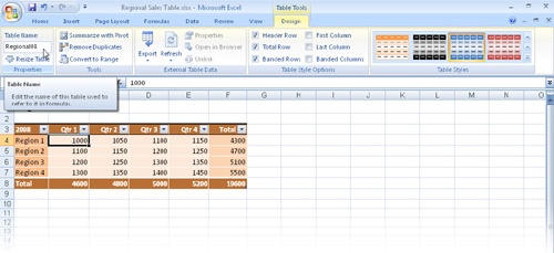
Structured references rely on the structure imposed when you create a table using the Table button on the Insert tab on the Ribbon. Excel recognizes distinct areas of a table as separate components you can refer to using specifiers that are either predefined or derived from the table. Figure 13-22 shows a modified version of the Regional Sales worksheet that we converted to a table. We’ll refer to this table as we discuss structured references.
When you refer to data in tables using formulas created by direct manipulation—that is, when you click or drag to insert cell or range references in formulas—Excel creates structured references automatically in most cases. (If a structured reference is not applicable, Excel inserts cell references instead.) Excel builds structured references using the table name and the column labels. (Excel automatically assigns a name to the table when you create one.) You can also type structured references using strict syntax guidelines that we’ll explain later in this section.
Note
The capability to create structured references automatically using direct manipulation with the mouse is an option that is ordinarily turned on. To disable this feature, click the Microsoft Office Button, Excel Options, and then in the Formulas category, clear the cryptically titled Use Table Names In Formulas check box.
All Excel tables contain the following areas of interest, as far as structured references are concerned:
The table. Excel automatically applies a table name when you create a table, which appears in the Table Name text box in the Properties group on the Table Tools Design tab that appears when you select a table. Excel named our table Table3 in this example, but we changed it to Regional08 by typing in the Table Name text box, as shown in Figure 13-22. The table name actually refers to all the data in the table, excluding the header and total rows.
Individual columns of data. Excel uses your column headers in column specifiers, which refer to the data in each column, excluding the header and the total row. A calculated column is a column of formulas inside the table structure, such as F4:F7 in our example, which, again, does not include the header or total rows.
Special items. These are specific areas of a table, including the total row, the header row, and other areas specified by using special item specifiers—fixed codes that are used in structured references to zero in on specific cells or ranges in a table. We’ll explain these later in this section.
No More Natural-Language Formulas
In previous versions of Excel, you could use adjacent labels instead of cell references when creating formulas, which was like using names without actually having to define them. This was called the natural-language formulas feature, but it was riddled with problems and has been replaced in Excel 2007 with structured references, which work much better. However, when you open a workbook created with a previous version of Excel containing natural-language formulas, the following, somewhat frightening, error message appears:
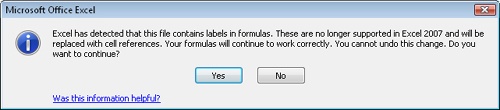
Despite the admonition that "Excel cannot undo this change," this mandatory conversion has little effect on your worksheets other than changing some of the underlying formulas. Excel correctly identifies the offending labels and replaces them for you with the correct cell references. If you still want your formulas to be more readable, you can then rebuild them using names or structured references.
Let’s look at an example of a structured reference formula. Figure 13-23 shows a SUM formula that we created by first typing =SUM(, then clicking cell B4, then typing another comma, and finally clicking cell C4. Because the data we want to use resides within a table and our formula is positioned in one of the same rows, Excel automatically uses structured references when we use the cursor to select cells while building formulas.

The result shown in the formula bar appears to be much more complex than necessary because we could just type =SUM(B4:C4) to produce the same result in this worksheet. But the structured formula is still quite easy to create using the mouse, and it has the distinct advantage of being able to automatically accommodate even the most radical changes to the table, which ordinary formulas are not nearly as good at accommodating.
Let’s examine a little more closely the structured reference contained within the parentheses of the SUM function shown in Figure 13-23. The entire reference string shown here is equivalent to the expression (B4,C4), which combines the cells on both sides of the comma. The portion of the reference string in bold represents a single, complete structured reference.
Regional08[[#This Row],[Qtr 1]],Regional08[[#This Row],[Qtr 2]])Here’s how the reference string breaks down:
The first item, Regional08, is the table specifier, which is followed by an opening bracket. Just like parentheses in functions, brackets in structured references always come in pairs. The table name is a little bit like a function, in that it always includes a pair of brackets that enclose the rest of the reference components. This tells Excel that everything within the brackets applies to the Regional08 table.
The second item, [#This Row], is one of the five special item specifiers and tells Excel that the following reference components apply only to those portions of the table that fall in the current row. (Obviously, this wouldn’t work if the formula were located above or below the table.) This represents an application of implicit intersection (see "Getting Explicit About Intersections").
The third item, [Qtr 1], is a column specifier. In our example, this corresponds to the range B4:B7. However, because it follows the [#This Row] specifier, only those cells in the range that happen to be in the same row as the formula are included, or cell B4 in the example.
The second reference follows the second comma in the string and is essentially the same as the first, specifying the other end of the range, or cell C4 in the example.
Here are some of the general rules governing the creation of structured references:
Table naming rules are the same as those of defined names. See "Naming Cells and Cell Ranges".
You must enclose all specifiers in matching brackets.
To make structured references easier to read, you can add a single space character in any or all of the following locations:
After the first opening (left) bracket (but not in subsequent opening brackets)
Before the last closing (right) bracket (but not in subsequent closing brackets)
After a comma
Column headers are always treated as text strings in structured references, even if the column header is a number.
You cannot use formulas in brackets.
You need to use double brackets in column header specifiers that contain one of the following special characters: tab, line feed, carriage return, comma, colon, period, opening bracket, closing bracket, pound sign, single quotation mark, double quotation mark, left brace, right brace, dollar sign, caret, ampersand, asterisk, plus sign, equal sign, minus sign, greater than symbol, less than symbol, and division sign; for example, Sales[[$Canadian]]. Space characters are permitted.
You can use three reference operators with column specifiers in structured references—a colon (:), which is the range operator; a comma (,), which is the union operator; and a space character ( ), which is the intersection operator.
For example, the following formula calculates the average combined sales for quarters 1 and 4 using a comma (the union operator) between the two structured references:
=AVERAGE(Regional08[Qtr 1],Regional08[Qtr 4])
The following formula calculates the average sales for quarters 2 and 3 by using colons (the range operator) to specify contiguous ranges of cells in each of the two structured references within the parentheses and by using a space character (the intersection operator) between the two structured references, which combines only the cells that overlap (Qtr 2 and Qtr 3):
=AVERAGE(Regional08[[Qtr 1]:[Qtr 3]] Regional08[[Qtr 2]:[Qtr 4]])
Excel provides five special codes you can use with your structured references that refer to specific parts of a table. You’ve already seen the special item specifier [#This Row] being used in previous examples. Here are all five special item specifiers:
[#This Row] This specifier identifies cells at the intersection created in conjunction with column specifiers; you cannot use it with any of the other special item specifiers in this list.
[#Totals] This refers to cells in the total row (if one exists) and otherwise returns a null value.
[#Headers] This refers only to cells in the header row.
[#Data] This refers only to cells in the data area between the header row and the total row.
[#All] This refers to the entire table, including the header row and the total row.
As you enter your formulas, the Formula AutoComplete feature is there to help you along by displaying lists of applicable functions, defined names, and structured reference specifiers as you type. For example, Figure 13-24 shows a formula being constructed using a SUM function, along with an AutoComplete drop-down list displaying all the defined items that are available that begin with the opening bracket character (also called a display trigger in AutoComplete parlance) that you just typed in the formula. Notice that the list includes all the column specifiers for the example table, as well as all the special item specifiers, all of which begin with a bracket.
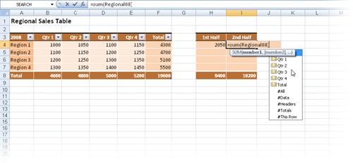
Figure 13-24. Structured reference specifiers automatically appear in the AutoComplete drop-down list if they are applicable when creating a formula.
To enter one of the items in the list in the formula, double-click it. The Formula AutoComplete list will most likely open more than once as you type formulas, offering any and all options that begin with the entered letters or display triggers. For example, the AutoComplete list appeared after we typed =S with a list of all the items beginning with that letter and again after typing the R in Regional08.
Note
For more information, see "Using Formula AutoComplete".
As a rule, structured references do not adjust like relative cell references when you copy or fill them—the reference remains the same. The exceptions to this rule occur with column specifiers when you use the fill handle to copy fully qualified structured references outside the table structure. For example, in the worksheet shown in Figure 13-25, we dragged the fill handle to copy the % of Total formula in cell K4 to the right, and the column specifiers in the formulas adjusted accordingly.

Figure 13-25. You can drag the fill handle to extend structured reference formulas into adjacent cells, but they behave a little bit differently than regular formulas.
The results illustrate some interesting structured reference behavior. Notice that the first formula shown in cell K4 divides the value in the Qtr 1 column by the value in the Total column. After we filled to the right, the resulting formula in cell N4 divides the value in the Qtr 4 column by the value in the Qtr 2 column. How did this happen?
As far as filling cells is concerned, tables act like little traps—you can check in, but you can’t check out. The top formula shown in Figure 13-25 has two column specifiers: Qtr 1 and Total. When we filled to the right, the Qtr 1 reference extended the way we wanted, extending to Qtr 2, Qtr 3, and Qtr 4 in each cell to the right. However, the Total reference, instead of extending to the right (G4, H4, I4) like a regular series fill would, "wrapped" around the table (2008, Qtr 1 and Qtr 2), resulting in the formula displayed in cell N4 at the bottom of Figure 13-25. This is interesting behavior, and we’re sure people will figure out ways to put it to good use.
What we need is a way to "lock" the Total column reference, but Excel doesn’t offer any way to create "absolute" column specifiers like we can with cell references. We can substitute a cell reference for the entire Total reference, as shown in Figure 13-26. We used a mixed reference in this case, specifying the absolute column $F but letting the row number adjust so we could fill down as well.

Figure 13-26. We replaced the second structured reference with an absolute cell reference to make filling these formulas work properly.
Note that if we were to select cell H4 in Figure 13-26 and drag the fill handle down, the formulas in each cell would not appear to adjust at all, and yet they would work perfectly. (The formula in cell H4 appears in Figure 13-23.) This is because explicit intersection, the built-in behavior of column specifiers, and the functionality of the [#This Row] specifier eliminate the need to adjust row references.