To save time, particularly when you are making entries into a large workbook with many formulas, you can switch from automatic to manual recalculation; that is, Excel will recalculate only when you tell it to do so. To set manual recalculation, click the Calculation Options button on the Formulas tab on the Ribbon, and choose the Manual option. You can also click the Microsoft Office Button, Excel Options, and then select the Formulas category to display the additional options shown in Figure 13-27.

Figure 13-27. The Formulas category in the Excel Options dialog box controls worksheet calculation and iteration.

Here are a few facts to remember about calculation options:

You might want to see the result of just one part of a complex formula if, for example, you are tracking down a discrepancy. To change only part of a formula to a value, select the part you want to change, and press F9. You also can use this technique to change selected cell references in formulas to their values. Figure 13-28 shows an example.

Figure 13-28. Select any part of a formula, and press F9 to convert it to its resulting value.

If you’re just verifying your figures, press the Esc key to discard the edited formula. Otherwise, if you press Enter, you replace the selected portion of the formula.

A circular reference is a formula that depends on its own value. The most obvious type is a formula that contains a reference to the same cell in which it’s entered. For example, if you type =C1-A1 in cell A1, Excel displays the error message shown in Figure 13-29. After you click OK, Excel opens the Help dialog box, which displays a pertinent topic.

Figure 13-29. This error message appears when you attempt to enter a formula that contains a circular reference.

If a circular reference warning surprises you, this usually means you made an error in a formula. If the error isn’t obvious, verify the cells that the formula refers to using the built-in formula-auditing features.

When a circular reference is present in the current worksheet, the status bar displays the text Circular References followed by the cell address, indicating the location of the circular reference on the current worksheet. If Circular References appears without a cell address, then the circular reference is located on another worksheet.

As you can see in Figure 13-30, when you click the arrow next to the Error Checking button on the Formulas tab and click Circular Reference, any circular references that exist on the current worksheet are listed on a menu that appears only if a circular reference is present. Click the reference listed on this menu to activate the offending cell.

Figure 13-30. The Circular References menu appears if any circular references are present.

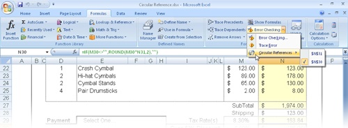
You can resolve many circular references. Some circular formulas are useful or even essential, such as the set of circular references shown in Figure 13-31. These formulas are circular because the formula in cell M30 depends on the value in M31, and the formula in M31 depends on the value in M30.

Figure 13-31. The discount formula in cell M29 is circular because it depends on the total, which in turn depends on the discount value in M29.

Figure 13-31 illustrates a useful circular reference scenario called convergence: The difference between results decreases with each iterative calculation. In the opposite process, called divergence, the difference between results increases with each calculation.

When Excel detects a circular reference, tracer arrows appear on the worksheet. To draw additional arrows to track down the source of an unintentional circular reference, select the offending cell, and then click Trace Precedents on the Formulas tab to draw tracer arrows to the next level of precedent cells, as shown in Figure 13-31.

You’ll find the Circular Reference.xlsx file in the Sample Files section of the companion CD.

After you dismiss the error message shown in Figure 13-29, the formula will not resolve until you allow Excel to recalculate in controlled steps. To do so, click the Microsoft Office Button, Excel Options, Formulas category, and in the Calculation Options section, select the Enable Iterative Calculation check box. Excel recalculates all the cells in any open worksheets that contain a circular reference.

If necessary, the recalculation repeats the number of times specified in the Maximum Iterations box (100 is the default). Each time Excel recalculates the formulas, the results in the cells get closer to the correct values. If necessary, Excel continues until the difference between iterations is less than the number typed in the Maximum Change text box (0.001 is the default). Thus, using the default settings, Excel recalculates either a maximum of 100 times or until the values change less than 0.001 between iterations, whichever comes first.

If the word Calculate appears in the status bar after the iterations are finished, more iterations are possible. You can accept the current result, increase the number of iterations, or lower the Maximum Change threshold. Excel does not repeat the "Cannot Resolve Circular Reference" error message if it fails to resolve the reference. You must determine when the answer is close enough. Excel can perform iterations in seconds, but in complex circular situations, you might want to set the Calculation option to Manual; otherwise, Excel recalculates the circular references every time you make a cell entry.

The Solver add-in, a "what-if" analysis tool, offers more control and precision when working with complex iterative calculations.

Here are three interesting facts about numeric precision in Excel:

Table 13-3 contains examples of how Excel treats integers and decimal fractions longer than 15 digits when they are typed in cells with the default column width of 8.43 characters.

Excel can calculate positive values as large as 9.99E+307 and approximately as small as 1.00E–307. If a formula results in a value outside this range, Excel stores the number as text and assigns a #NUM! error value to the formula cell.