A.1 INTRODUCTION

Matrix algebra provides at least two important advantages: (1) it enables reducing complicated systems of equations to simple expressions that can be visualized and manipulated more easily, and (2) it provides a systematic, mathematical method for solving problems that is well adapted to computers. Problems are frequently encountered in surveying, geodesy, and photogrammetry that require the solution of large systems of equations. This book deals specifically with the analysis and adjustment of redundant observations that must satisfy certain geometric conditions. This frequently results in large equation systems, which when solved according to the least squares method yield most probable estimates for adjusted observations and unknown parameters. As will be demonstrated, matrix methods are particularly well suited for least squares computations, and in this book they are used for analyzing and solving these equation systems.

A.2 DEFINITION OF A MATRIX

A matrix is a set of numbers or symbols arranged in a square or rectangular array of m rows and n columns. The arrangement is such that certain defined mathematical operations can be performed in a systematic and efficient manner. As an example of a matrix representation, consider the following system of three linear equations involving three unknowns:

(A.1)

In Equation (A.1), a's are the coefficients of the unknown parameters x, and c's the constant terms. The system above can be represented in summation notation as

It can also be represented in matrix form as

(A.2)

In turn, Equation (A.2) can be represented in compact matrix notation as

(A.3)

In Equation (A.3), capital letters (A, X, and C) are used to denote a matrix or an array of numbers or symbols. From simplified Equation (A.3), it is immediately obvious that matrix methods provide a compact shorthand notation convenient for handling large systems of equations.

A.3 SIZE OR DIMENSIONS OF A MATRIX

The size or dimension of a matrix is specified by its number of rows m and its number of columns n. Thus, the following matrix ₂D³ is a 2 × 3 matrix where there are two rows and three columns (i.e., m = 2, n = 3). Notice that the subscript indicates the number of rows and the superscript indicates the number of columns in the notation ₂D³.

Also, the matrix E below is a 3 × 2 matrix

Note that the position of an element in a matrix is defined by a double subscript, and that a lowercase letter is used to designate any particular element within a matrix. Thus, d₂₃ = 1 is in row 2 and column 3 of the above matrix D. In general, the subscript ij indicates an element's position in a matrix where i represents the row and j the column.

A.4 TYPES OF MATRICES

Several different types of matrices exist as described below. Various symbols can be used to designate them as illustrated.

1. Column matrix. The number of rows can be any positive integer, but the number of columns is one. This matrix is also known as a vector.
   
2. Row matrix. The number of columns can be any positive integer but the number of rows is one.
   
3. Rectangular matrix. The number of rows and columns are m and n, respectively, where m and n are any positive integers.
   
4. Square matrix. The number of rows equals the number of columns.
   

A square matrix, for which the determinant is zero, is termed singular. If the determinant is nonzero it is termed nonsingular (the determinant of a matrix is discussed in Section B.3).

5. Symmetric matrix. The matrix is mirrored about the main diagonal going from top left to bottom right (i.e., element a_ij = element a_ji). A symmetric matrix is always a square matrix.
   
6. Diagonal matrix. Only the elements on the main diagonal are not zero. The diagonal matrix is always a square matrix.
   
7. Unit matrix. A diagonal matrix with ones along the main diagonal. It is also called the identity matrix and is usually identified by the symbol I.
   
8. Transpose of a matrix. It is obtained by interchanging rows and columns (i.e., element = element a_ji). Thus, the dimensions of A^T are the reverse of the dimensions of A. If
   

the transpose of A, denoted A^T is

A.5 MATRIX EQUALITY

Two matrices are said to be equal only when they are equal element by element. Thus, the two matrices must be the same size or have the same dimensions.

A.6 ADDITION OR SUBTRACTION OF MATRICES

Matrices can be added or subtracted, but to do so, they must have the same dimensions. If two matrices have equal dimensions, they are said to be conformable for addition or subtraction. In adding or subtracting matrices, elements from each unique row/column position of the two matrices are added or subtracted systematically. The sum or difference is placed in the same unique row/column location of the resulting matrix. The following example illustrates this procedure.

Assuming that two matrices are conformable for addition or subtraction, the following are true:

A.7 SCALAR MULTIPLICATION OF A MATRIX

Matrices can be multiplied by a scalar (i.e., a constant). Let k be any scalar quantity; then

The following are examples

As illustrated in the example above, each element of the matrix A is multiplied by the scalar k to obtain the elements of C. Note that 4 × A = A + A + A + A = A × 4.

A.8 MATRIX MULTIPLICATION

If matrix A is to be post-multiplied by matrix B (i.e., the product of AB determined, the number of columns in matrix A must equal the number of rows in matrix B). This is a basic requirement for matrix multiplication. When this condition is satisfied, the two matrices are said to be conformable for multiplication. The product C will have the same number of rows as A and the same number of columns as B. Thus, the following multiplications are possible:

These multiplications are not possible:

To demonstrate the process of matrix multiplication, consider the following example:

The elements c_ij of matrix C are the total sums obtained by successively multiplying each element in row i of matrix A by the elements in column j of matrix B, and then summing these products. Thus, for the example above,

The process above is seen more easily with a numerical example.

The student should now verify the matrix representation of Equations (A.1) and (A.2). Notice that the product of a unit matrix, I, and a conformable matrix, A (one with the same number of rows as I), equals the original matrix A. Thus,

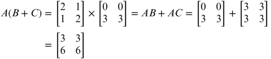
Assuming that matrices A, B, and C are conformable for multiplication and in the order indicated, then the following are true.

1. (c) A(B+C) = AB + AC   (first distributive law)
2. (d) (A+B)C = AC + BC   (second distributive law)
3. (e) A(BC) = (AB)C          (associative law)
4. (f) (AB)^T = B^TA^T

The following cautions are also stated:

1. (g) AB is not generally equal to BA, and BA may not even be conformable for multiplication.
2. (h) If AB = 0, neither A nor B are necessarily = 0.
3. (i) If AB = AC, B does not necessarily = C.

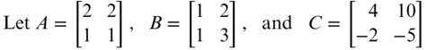
Let

Example of (c):

Example of (d)¹:

Example of (e):

Example of (f):

so

Example of (g):

Example of (h):

Then AB = 0, but neither A nor B equal 0.

Example of (i):

Then AB = AC, but B ≠ C, where

A.9 COMPUTER ALGORITHMS FOR MATRIX OPERATIONS

It should be apparent that addition, subtraction, and multiplication of large matrices involve many arithmetic operations. These are very tedious when done by hand, but can be done quickly by a computer. In this section, general mathematical expressions are developed for performing these operations using a computer. These general mathematical expressions, when programmed for computer solution, are called algorithms.

A.9.1 Addition/Subtraction of Two Matrices

Consider the two matrices A and B that are shown in Figure A.1. Note that matrices A and B are conformable for addition. Find the sum of the two matrices and place the results in C.

• Step 1: Add the first element (a₁₁) of the A matrix to the first element (b₁₁) of B, placing the result in the first element (c₁₁) of C. Repeat this process for each of the successive columns along the first row of A and B or from j = 1 to j = n.
• Step 2: Iterate step 1 for each successive row of the matrices, or for rows increasing from i = 1 to i = m. Table A.1 shows this entire operation of adding two matrices in the four computer languages of BASIC, C, FORTRAN, and Pascal.

BASIC Language 1000 For i = 1 to M 1010 For j = 1 to N 1020 C(i,j) = A(i,j) + B(i,j) 1030 Next j 1040 Next i	FORTRAN Language Do 100 I = 1,M Do 100 J = 1,N C(i,j) = A(i,j) + B(i,j) 100 Continue
C Language for (i=0; i<m; i++) for (j=0; j<n; j++) C[i][j] = A[i][j] + B[i][j];	Pascal Language For i := 1 to M do For j := 1 to N do C[i,j] := A[i,j] + B[i,j];

A.9.2 Matrix Multiplication

Consider the two matrices A and B that are shown in Figure A.2. Again, these matrices, A and B, are conformable for multiplication. Find the product AB and place the results in C.

• Step 1: Sum the products (A row i = 1) × (B column k = 1), with the elements of A and B being increased successively from j = 1 to j = p. Place the result in c_ik, or c₁₁, for the first step. Mathematically, this step is represented as:
  
• Step 2: Increase k successively by 1, repeat step 1, and place the results in c_ik. Continue increasing k and repeating step 1 until k = p.
• Step 3: Increase i from one to two, and repeat steps 1 and 2 in entirety. Upon completion with i = 2, increment i by one and repeat steps 1 and 2 again in entirety. Continue this process through i = m. This completes the matrix multiplication.

BASIC Language For i = 1 to M For k = 1 to N C(i,k) = 0.0 For j = 1 to P C(i,k) = C(i,k) + A(i,j)*B(j,k) Next j : Next k: Next I	FORTRAN Language Do 100 I = 1,M Do 100 K = 1,N C(i,k) = 0.0 Do 100 J = 1,P C(i,k)=C(i,k)+A(i,j)*B(j,k) 100 Continue
C Language for (i=0; i<m; i++) for (k=0; k<n; k++) { C[i][k] = 0; for (j=0; j<p; j++) C[i][k] = C[i][k] + A[i][j]*B[j][k]; } //for k	Pascal Language For i := 1 to M do For k := 1 to N do Begin C[i,k] := 0.0; For j := 1 to P do C[i,k] := C[i,k] + A[i,j]*B[j,k] End; { for k }

This operation is shown Table A.2 in the four languages of BASIC, C, FORTRAN, and Pascal. As a final note on multiplication, it is essential that the order in which the matrices are multiplied be specified.

A.10 USE OF THE MATRIX SOFTWARE

A software package called MATRIX is included on the companion website that is provided with this book. It includes all the matrix operations that will be necessary to study the subject of adjustment computations and solve the after-chapter problems herein that require matrix manipulation. Instructions for use of the software are given in the help file, which is part of the software.

MATRIX reads the matrices from text files and contains a text editor to create such files. The files are free format, which means that a space, comma, or tab can separate each entry. This also means that commas cannot be used as thousand's separators in a single large number. Although the internal editor in MATRIX does not support tabs, a tab entry can be used to separate entries also. This feature is useful when cutting and pasting matrices from a spreadsheet. A file of matrices from Section A.8, which were used to demonstrate principles (c) and (d), is shown in Figure A.3 where the format of the files is

1. Job title.
2. Matrix name.
3. Number of rows and columns in matrix.
4. List each element in the first row.
5. Continue in the same manner for each subsequent row, by placing each row of a matrix on a new line.
6. Repeat the lines 2 through 5 for each matrix.

After creating the file, it must be saved and read into the MATRIX software shown in Figure A.4 using the read file option under the matrices menu of the software. Once read into the software, the user can perform any of the matrix operations contained in the numerical operations menu. When an operation is selected, a matrix selection screen will appear. Figure A.5 shows the selection screen after the multiplication option has been selected. Note that the previous addition of matrices A and B are shown as A + B and the directions to the user shown at the top of the screen where it states select the first matrix A in the product of AB. There is a rename option under the matrices menu that allows the user to change the default name of a matrix to any name up to 20 characters long. Two options in the numerical operations menu allow the user to perform both a weighted and unweighted least squares adjustment as discussed in Chapter 11. These options create all of the intermediate matrices that are necessary to perform the adjustment and compute the post-adjustment statistics as presented in Chapter 13.

Users can view the results any of the matrices using the view matrix option in the matrices menu. This option can be also accessed with the short-cut key ctrl-v. The number of digits after the decimal point can be controlled by using the display options under the matrices menu. For example, since the additions of Section A.8 involved only integers, the user may select zero digits after the decimal point so that integers are displayed. To print the resulting matrices, the user simply needs to select the list matrix option in the matrices menu. The user will be prompted for the location and name of the resulting file, which will be created to list the selected matrices. When this option is used, the user can select multiple matrices from the matrix selection screen. These matrices will be written to the user-specified file using the display option specified digits after the decimal point. Once saved, this file can be read into the MATRIX editor and printed. The write file option in matrices menu allows the user to create a text file, which is readable by MATRIX, of all the matrices shown in the selection screen. The matrices will be written in scientific notation so that no accuracy is lost between the saving and reading of the resultant file.

PROBLEMS

1. A.1 Represent the following system of linear equations in matrix form as AX = B.
   
2. A.2 For Problem A.1, find the product of A^TA.
3. A.3 Do the following matrix operations
   1. (a)
   2. (b)
   3. (c)
   4. (d)
4. A.4 Solve Problem A.2 using the MATRIX software.
5. A.5 Solve Problem A.3 using the MATRIX software.
6. A.6 Let
   1. (a) Find AB.
   2. (b) Find B².
   3. (c) Find CB.
   4. (d) Find BA.
   5. (e) Find B³.
   6. (f) Find DB.
   7. (g) Find C³.
7. A.7 Do Problem A.6 using the MATRIX software.
8. A.8 Multiply the following, if possible. If not possible, give reasons why the multiplication cannot be done.
   1. (a)
   2. (b)
   3. (c)
   4. (d)
9. A.9 Expand the following summations into their equivalent algebraic expressions.
   1. (a)
   2. (b)
   3. (c)
   4. (d)
   5. (e)
   6. (f)
10. A.10 Write the algebraic expressions for the system of equations represented by the following matrix notation.
    
11. A.11 Show that in general, (AB)^T = B^TA^T.

PROGRAMMING PROBLEMS

1. A.12 Write a program that will read and write the elements of a matrix, compute the transpose of the matrix, and write the solution. (Hint: Place the reading, writing, and transposition codes in separate subroutines/procedures/functions to be called from the main program.)
2. A.13 Select one of the matrix addition codes from Table A.1 and enter it and any necessary supporting code to solve Problem A.3(a). (Hint: Place the code in Table A.1 in a separate subroutine/procedure/function to be called from the main program.)
3. A.14 Select one of the matrix multiplication programs from Table A.2, and enter this code and any necessary supporting code to solve Problem A.3(d). (Hint: Place the code in Table A.2 in a separate subroutine/procedure/function to be called from the main program.)
4. A.15 Write a program that will read and write a file of matrices, and do the matrix operations of transposition, addition, subtraction, and multiplication. Demonstrate the program by doing Problems A.2 and A.3 (a), (b), and (d). (Hint: Place the reading, writing, transposition, addition, subtraction, and multiplication, codes in separate subroutines/procedures/functions to be called from the main program.)
5. A.16 Write a Mathcad worksheet that solves Problems A.3 and A.6.