4

Instruction Scheduling Before Register Allocation

Since controlling the register pressure during instruction scheduling is a difficult problem, lifetime-sensitive modulo schedulers have been proposed [HUF 93a], which aim at minimizing the cumulative register lifetimes. In this chapter, we show that in the case of resource-free modulo scheduling problems, the modulo schedule that minimizes the cumulative register lifetimes is easily computed by solving a network flow problem on the dependence graph suitably augmented with nodes and arcs.

4.1. Instruction scheduling for an ILP processor: case of a VLIW architecture

As a case of interest, this section presents instruction scheduling for the ST200 architecture.

4.1.1. Minimum cumulative register lifetime modulo scheduling

The minimization of the cumulative register lifetimes on the sample dependence graph is illustrated in Figure 4.1. This dependence graph has been simplified by removing the memory access operations after converting the uniform dependences into register transfers [CAL 90]. We assume that the target architecture is such that the lifetime of a register starts at the time when the operation that produces it is issued. When this is not the case, the only difference is a constant contribution to the cumulative register lifetimes that does not impact the minimization.

Figure 4.1. Original dependence graph

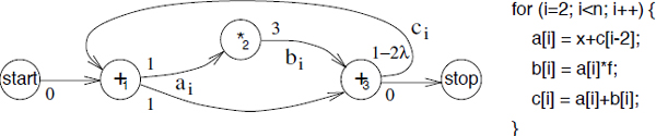
Taking the dependence graph in Figure 4.1, let be the schedule dates of the respective operations +₁, *₂, +₃ and let be the lifetimes of the register defined by these operations [DIN 94]. Then we get the following system of inequalities:

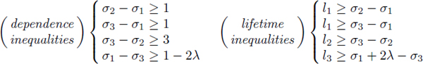
This illustrates the equations we introduced in [DIN 94] and the minimum cumulative register lifetimes (MCRL) problem is defined with the objective to minimize Σ_i l_i. In [DIN 96], we introduced a transformation of the MCRL problem that makes it solvable in a simple and efficient way. The first step is to introduce the variables such that and to eliminate the variables :

Figure 4.2. Augmented dependence graph

This new system of inequalities defines an augmented dependence graph, which is derived from the dependence graph as follows: any register lifetime producer node is paired with a lifetime node and for any lifetime arc between the producer node and a consumer node, we add an arc from the consumer node to the lifetime node. This transformation is illustrated in Figure 4.2 for the dependence graph in Figure 4.1. Since , the objective to minimize Σ_i l_i becomes Σ_i r_i – α_i.

It is interesting to compare these equations to those of the minimum buffers problem, as defined by Ning and Gao [NIN 93b]. In the minimum buffers problem, the so-called buffer variables are defined and the objective is to minimize Σ_i b_i:

Obviously, the dependence equations are the same, while the buffer and the lifetime equations are different, although related. To make the minimum buffers problem easier to solve, Ning and Gao [NIN 93b] make the change of variables ; so the left-hand side of the buffer inequalities become identical to the left-hand side of the lifetime inequalities.

The MCRL problem is efficiently solved on the augmented dependence graph [DIN 96]. To see how, let us first assume that all the arcs of the original dependence graph carry a lifetime. Then, if U denotes the arc-node incidence matrix of the original dependence graph, the primal-dual relationships of linear programming can be written as:

Here, the linear program associated with the MCRL problem appears on the left and its dual on the right. Negating both sides of the equal sign in the dual linear program yields a maximum-cost network flow problem on the dependence graph augmented with the lifetime nodes, where each producer node supplies unit flow and where each lifetime node demands unit flow. In practice, only the nodes of the dependence graph that define a register are paired with a lifetime node.

Beyond the MCRL problems, the generalization of a resource-free scheduling problem, which is solved as a single-source longest path over the dependence graph, into a maximum cost network flow problem over the augmented dependence graph allows the introduction of “soft constraints” in instruction scheduling problems. In the STMicroelectronics ST100 linear assembly optimizer (LAO) code generator [DIN 00], increasing some of the flow requirements addressed the non-standard instruction scheduling features of the ST120 decoupled implementation. The augmented dependence graph is also used for the time-indexed integer linear programming formulations of the register pressure instruction scheduling problems (see section 4.1.6).

4.1.2. Resource modeling in instruction scheduling problems

The resource constraints for instruction scheduling on a very long instruction word (VLIW) processor are described in a micro-architecture manual by a set of admissible bundles, that is, combinations of operations that may issue without resource conflicts¹. More precisely, a bundle is a sequence of resource classes, where each resource class is an abstraction for the resource requirements of the operations in the instruction scheduling problem. Going from the bundle specifications of a processor to an accurate model with cumulative resources is not guaranteed to succeed. Techniques to build the cumulative resource model, given a processor description, are described in [RAJ 00, RAJ 01]. Their idea is to introduce artificial resources where required, based on the identification of critical sets of resource classes.

Even with the introduction of artificial resources like ODD for the ST220 in Figure 2.1, a processor cumulative resource model can still be an approximation because the cumulative constraints can only represent convex regions of resource classes. To illustrate this point, consider a processor with two resource classes A, B and an issue width of 4. Then, no cumulative resource constraints may allow the combinations {A, A, A, B} and {A, B, B, B} while disallowing the combinations {A, A, B, B}. Indeed, this yields the contradiction 3a + b ≤ c ∧ a + 3b ≤ c ∧ 2a + 2b > c, assuming that a and b are the resource requirements of A and B and that c is the resource availability.

Another limitation of the cumulative resources model is that all the resources involved in the execution of an operation O_i are assumed busy for its whole processing time p_i. Thus, when two operations O_i and O_j need to share an exclusive resource, either σ_i + p_i ≤ σ_j or σ_j + p_j ≤ σ_i. To increase the precision of resource modeling, we need to express the fact that given an exclusive resource, either σ_i + or σ_j + ≤ σ_i, where and both depend on O_i and O_j. The interpretation of is the minimum number of cycles between σ_i and σ_j that ensures there are no resource conflicts between O_i and O_j, assuming O_i is scheduled before O_j. Such resource constraints can be modeled with regular reservation tables.

Figure 4.3. A reservation table, a regular reservation table and a reservation vector

A regular reservation table is the traditional Boolean pipeline reservation table of an operation [KOG 81, RAU 96], with the added restrictions that the ones in each row start at column zero and are all adjacent. In the case of exclusive resources, the regular reservation tables are also equivalent to reservation vectors. Figure 4.3 illustrates the representation of conditional store operation of the DEC Alpha 21064 using a reservation table, a regular reservation table and a reservation vector. The regular reservation tables are accurate enough to cover many pipelined processors. For example, when describing the DEC Alpha 21064 processor, we found [DIN 95] that the regular reservation tables were slightly inaccurate only for the integer multiplications and the floating-point divisions.

A main advantage of regular reservation tables is that expressing the modulo resource constraints yields inequalities that are similar to the dependence constraints. Let us assume a resource-feasible modulo scheduling problem at period λ and two operations O_i and O_j that conflict on an exclusive resource. Then, 1 ≤ , ≤ λ and the dates when operation O_i uses the exclusive resource belong to . In the modulo scheduling problem, O_i and O_j do not conflict iff , that is:

This result is similar to inequalities [2.2] given by Feautrier [FEA 94] for the exclusive constraints of D-periodic scheduling, with the refinement that we express the value of given σ_i and σ_j.

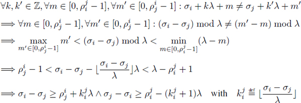
4.1.3. The modulo insertion scheduling theorems

Insertion scheduling [DIN 95] is a modulo scheduling heuristic that builds a series of partial modulo schedules by starting from a resource-free modulo schedule and by adding dependences or increasing λ to resolve the modulo resource conflicts until a complete modulo schedule is obtained. A partial modulo schedule is a modulo schedule where all the dependences are satisfied, while some of the resource conflicts are ignored. Insertion scheduling relies on conditions for transforming a partial modulo schedule {σ_i}_1≤i≤n at period λ into another partial modulo schedule {σ′_i }_1≤i≤n at period λ′. To present these conditions, we first define {ϕ_i, τ_i, ϕ′_i, τ′_i, δ_i}_1≤i≤n such that:

[4.1]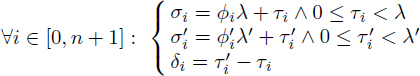

We are interested in modulo schedule transformations where ∀i ∈ [1, n] : ϕ′_i = ϕ_i, τ_′i = τ_i + δ_i and δ_i < ∆ with . Let O_i O_j denote the fact that O_i precedes O_j in the transitive closure of the loop-independent dependences ( = 0) of the dependence graph². The following result states the conditions that must be met by the δ_i in order to preserve all the dependence constraints:

THEOREM 4.1.– Let {σ_i}_1≤i≤n be a dependence-feasible modulo schedule of a modulo scheduling problem P at period λ. Let {σ′_i}_1≤i≤n be n integers such that:

[4.2]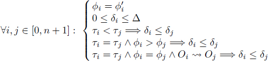

Then {σ′_i}_1≤i≤n is a dependence-feasible modulo schedule of P at period λ + ∆.

PROOF.– Let be a dependence of P. From the definition of a dependence constraint, , or equivalently .

Given the hypothesis [4.2], let us show this dependence holds for {σ′_i}_1≤i≤n, that is, .

Dividing the dependence inequality by λ and taking the floor yields ϕ_j – ϕ_i + , since all values are non-negative. We have 0 ≤ τ_i < λ, 0 ≤ τ_j < λ; hence, 0 ≤ |τ_j – τ_i | < λ and the value of is –1 or 0. Therefore, ϕ_j – ϕ_i ≥ – and we consider its subcases:

ϕ_j – ϕ_i = –: Let us show that τ′_j – τ′_i ≥ .

Since ≥ 0, we have τ_j ≥ τ_i. Several subcases need to be distinguished:

τ_i < τ_j: From [4.2], we have .

τ_i = τ_j ∧ ϕ_i ≠ ϕ_j: Either ϕ_i > ϕ_j or ϕ_i < ϕ_j. The latter is impossible, for = ϕ_i – ϕ_j and since all are non-negative. From [4.2], τ_i = τ_j ∧ ϕ_i > ϕ_j yields δ_j > δ_i; therefore, the conclusion is the same as above.

τ_i = τ_j ∧ ϕ_i = ϕ_j: Since = ϕ_i – ϕ_j = 0, there are no dependence constraints unless O_i O_j. In this case, taking δ_i ≥ δ_j works like in the cases above.

ϕ_j – ϕ_i > –: Let us show that (ϕ_j – + ϕ_i + )λ′ + τ′_j – τ′_i – ≥ 0.

We have ϕ_j – ϕ_i + ≥ 1, so (ϕ_j – ϕ_i + )λ′ ≥ (ϕ_j – ϕ_i + )λ + ∆. From [4.2] , we also have τ_i ≤ τ′_i ≤ τ_i + ∆ and τ_j ≤ τ′_j ≥ τ_j + ∆, so τ′_j – τ′_i ≥ τ_j – τ_i – ∆. Hence, (ϕ_j – ϕ_i + )λ′ + τ′_j – τ′_i – ≥ (ϕ_j – ϕ_i + )λ + ∆ + τ_j – τ_i – ∆ – = (ϕ_j – ϕ_i + )λ + τ_j – τ_i – ≥ ⁰.

COROLLARY 4.1.– In a dependence-feasible modulo schedule {σ_i}_1≤i≤n, for any dependence , then:

A result similar to theorem 4.1 holds for the modulo resource constraints of a modulo schedule, assuming these constraints only involve regular reservation tables and exclusive resources.

THEOREM 4.2.– Let {σ_i}_1≤i≤n be schedule dates satisfying the modulo resource constraints at period λ, assuming regular reservation tables and exclusive resources. Let {σ′_i}_1≤i≤n be such that:

[4.3]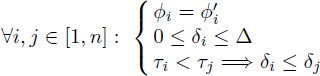

Then {σ′_i}_1≤i≤n also satisfies the modulo resource constraints at period λ + ∆.

PROOF.– With the regular reservation tables, the modulo resource constraints at A for the schedule dates σ_i, σ_j of two operations O_i, O_j that need the exclusive resource are equivalent to (see section 4.1.2):

[4.4]

These constraints look exactly like ordinary dependence constraints, save the fact that the ω values are now of arbitrary sign. Since the sign of the ω values is only used in the proof of theorem 4.1 for the cases where τ_i = τ_j, which need not be considered here because they imply no resource conflicts between σ_i and σ_j, we deduce from the proof of theorem 4.1 that {σ′_k}_1≤k≤n satisfies the modulo resource constraints at period λ′.

THEOREM 4.3.– Let {σ_i}_1≤i≤n be schedule dates satisfying the modulo resource constraints at period λ, assuming cumulative resources. Then, under the conditions [4.3], {σ′_i}_1≤i≤n also satisfies the modulo resource constraints at period .

PROOF.– In the proof of theorem 4.2, whenever [4.4] holds for {σ_i}_1≤i≤n, it holds under the conditions [4.3] for {σ′_i}_1≤i≤n, for any assumed values of and . This ensures that the simultaneous use of the cumulative resources does not increase in σ′_i}_1≤i≤n.

By theorem 4.1 and corollary 4.3, any transformation of a partial modulo schedule {σ_i}_1≤i≤n at period λ into {σ′_i}_1≤i≤n at period , under the conditions [4.2] , yields a partial modulo schedule.

4.1.4. Insertion scheduling in a backend compiler

Insertion scheduling [DIN 95] is a modulo instruction scheduling heuristic that issues the operations in a given priority order, where the issuing of an operation is materialized in the dependence graphs by adding dependence arcs to constrain the feasible schedule dates of this operation to be exactly its issue date. In addition, insertion scheduling applies the insertion theorems of section 4.1.3 to resolve the resource conflicts between the previously issued operations and the current operation to issue by increasing the period λ to make room for this operation. Under its simplest form, insertion scheduling relies on single-source longest path computations like most scheduling heuristics.

The ST200 LAO instruction scheduler implementation, however, uses MCRL minimization to achieve lifetime-sensitive instruction scheduling (section 4.1.1). To solve the MCRL problems, this implementation relies on a network simplex algorithm to optimize the maximum cost flow problems [AHU 93] and on a network simplex longest path algorithm to find the initial solutions [GOL 91]. Besides being efficient in practice [DIN 96], the network simplex algorithms maintain the explicit values of the primal (edge flows) and the dual (node potentials) variables. The latter are precisely the schedule dates of the operations. The ST200 LAO implementation of insertion scheduling is as follows:

Step 0 The resource-free MCRL modulo scheduling problem, called P₀, is built and solved. This problem is represented MCRL by the forward dependence graph, the backward dependence graph and the MCRL augmented graph. We solve P₀ with a network simplex longest path algorithm, followed by a dual network simplex algorithm. The network simplex longest path algorithm starts with A the period set to the lower bound λ_res and solves the optimum cost to time ratio problem by increasing the period to λ_rec if necessary for P₀ feasibility.

Step j This step transforms the modulo scheduling problem P_j–1 into P_j. Let denote the issue dates assigned to the operations {O_ik }_{1≤k≤j–1} in the previous steps, that is . The not yet issued operations are ranked in priority order and the operation with the highest priority, denoted by O_ij , is issued as follows:

1) Run a primal network simplex algorithm on three dependence graphs to compute the early start date e_ij, the late start date l_ij and the MCRL date m_ij, of O_ij in P_j–1. Then, compute and . The possible issue dates are scanned first in [m_ij, m_ij + a_ij ] in increasing order and second in [m_ij – b_ij, m_ij – 1] in decreasing order. This ensures that no more than λ feasible dates are scanned and the issue dates next to the MCRL date m_ij are scanned first.

2) Select as the first scanned date with the lowest modulo resource conflicts between O_ij and {O_ik }_{1≤k≤j–1}. This is measured by the minimum number of cycles ∆; the period λ_j–1 needs to increase to remove the modulo resource conflicts at period . If there are no conflicts between O_ij and {O_ik }_{1≤k≤j–1} for σ_ij = , then ∆ = 0.

3) Let _1≤k≤j be the issue dates in P_j–1, and _1≤k≤j be the issue dates in P_j. The issue dates in P_j are computed from the issue dates in P_j–1 by applying theorem 4.1, with {δ_ik }_{1≤k≤j–1} chosen to eliminate the modulo resource constraints between O_ij and {O_ik }_{1≤k≤j–1}. See [DIN 95] for the details of the δ_ik computations.

4) Build the modulo scheduling problem from and the {δ_ik }_1≤k≤j and update the modulo resource table.

At the end of step j, all the dependence constraints are satisfied, as are the modulo resource constraints for the operations {O_ik }_1≤k≤j. At the end of step n, a modulo schedule is available.

In the ST200 LAO instruction scheduler, insertion scheduling operates both in prepass and postpass instruction scheduling and the instruction scheduling regions are super blocks. During prepass scheduling, the lifetime-sensitive scheduling is enabled and the inner loops are either modulo scheduled or loop scheduled. In postpass scheduling, the lifetime-sensitive scheduling is disabled and all inner loops, including the software pipelines created during prepass scheduling, are loop scheduled. Loop scheduling is a restricted form of modulo scheduling, where the period is exactly the same as the local schedule length. This is achieved by adding a dependence O_n+1 → O₀ with latency 1 and distance 1 to the P₀ problem. As a result, loop scheduling accounts for the effects of the loop-carried dependences, while preventing code motion between the loop iterations.

4.1.5. Example of an industrial production compiler from STMicroelectronics

The STMicroelectronics ST200 production compiler st200cc is based on the GCC compiler frontend components, the Open64 compiler technology [OSG 13], the ST200 LAO global instruction scheduler adapted from the ST100 LAO code generator [DIN 00], an instruction cache optimizer [BID 04] and the GNU backend tools. The Open64 compiler has been retargeted from the Intel IA64 to the STMicroelectronics ST200 architecture, except for the instruction predication, the global code motion (GCM) instruction scheduler and the software pipeliner (SWP). Indeed, these components appeared to be too dependent on the IA64 architecture predicated execution model and on its support of modulo scheduling through rotating register files.

In the st200cc compiler, the Open64 GCM and SWP components are replaced by the ST200 LAO instruction scheduler, which is enabled at optimization level -03. At compiler optimization level -02 and below, only the Open64 basic block instruction scheduler is active. The ST200 LAO instruction scheduling and software pipelining relies on the following techniques:

– A transactional interface between the Open64 code generator intermediate representation (CGIR) and the LAO intermediate representation (LIR).

– Parsing of the control flow graph into a loop nesting forest and super block formation. The super block formation does not include tail duplication [HAN 93], as this is performed in the Open64 code generator by the ST200-specific instruction predication.

– Prior to prepass and postpass scheduling, the algorithm of Leung et al. [LEU 01] is iterated over each resource of the ST220 model (Figure 2.1), starting with the more heavily used resources. This iteration starts with the period set to the minimum value λ_res such that the renewable resources are not oversubscribed; then, the period is increased until the relaxation is feasible.

– Prepass instruction scheduling based on insertion scheduling, which performs lifetime-sensitive superblock scheduling, loop scheduling and modulo scheduling. The scheduling order is the lower MCRL dates first and the scheduling priorities are the modified deadlines computed by the scheduling algorithm of Leung et al. [LEU 01].

– Postpass instruction scheduling based on insertion scheduling, which performs block scheduling and loop scheduling. The scheduling order is the lower consistent release dates first and the scheduling priorities are the modified deadlines computed by the scheduling algorithm of Leung et al. [LEU 01].

Figure 4.4. Counted loop software pipeline construction with and without preconditioning

Once a modulo schedule is available, it must be transformed into a software pipeline. In Figure 4.4, we illustrate the classic software pipeline construction for the local schedule of a counted loop that spans five stages named A, B, C, D and E. In the basic case (a), loop preconditioning [RAU 92b] is required to ensure that the software pipeline will execute enough iterations to run the prologue and the epilogues. Without preconditioning, case (b) software pipeline construction is required. In the embedded computing setting, these classic software pipeline construction schemes are not effective because they only apply to counted loops and involve significant code size expansion.

For the ST200 modulo scheduling, we construct all software pipelines like while-loops, as illustrated in Figure 4.5(a). This while-loop construction scheme speculatively starts executing the next iterations before knowing if the current iteration is the last iteration and relies on the dismissible loads of the ST200 architecture. Another refinement implemented in the ST200 LAO is induction variable relaxation [DIN 97a] and the restriction of modulo expansion to variables that are not live on loop exit. As a result, epilogues are unnecessary for virtually all the software pipelines.

Figure 4.5. While-loop software pipeline construction without and with modulo expansion

Modulo expansion is a technique introduced by Lam [LAM 88a], where the non-RAW register dependences on variables are omitted from the dependence graph. This exposes more parallelism to the modulo scheduler, but when the software pipeline is constructed, each such variable may require more than one register for allocation. Modulo renaming is supported by architectures like the IA64 through rotating registers [RAU 92a]. On architectures without rotating registers like the ST200, modulo expansion is implemented by kernel unrolling [LAM 88a, DIN 97a, LLO 02], as illustrated in case (b) of Figure 4.5.

To compare the effects of the instruction scheduling techniques available for the ST220 processor, we use the benchmark suite collected by the Hewlett Packard (HP) Laboratories for embedded computing and we also include the performances of the HP/Lx multiflow-based compiler. This compiler implements trace scheduling [LOW 93] and targets the ST200 architecture including the ST220 processor. In Figure 4.6, we compare the performance in cycles and without the cache miss effects of the multiflow-based compiler at optimization level -03 (MF), the st200cc compiler at -03 with software pipelining disabled (O3-nopipe), and the st200cc at -03 that enables software pipelining by default (O3). All the performances in Figure 4.6 are normalized by those of st200cc compiler at -03 with the ST200 LAO disabled, where basic block scheduling is done in prepass and postpass by the Open64.

When enabling the ST200 LAO block scheduling and loop scheduling on super blocks, the geometric mean improvement is 5.5%, compared to the reference. When enabling the ST200 LAO software pipelining, the geometric mean improvement is 9.5%. This progression illustrates the benefits of the LAO super block scheduling over the Open64 basic block scheduling and the significant performance benefits brought by software pipelining. Due to the while-loop software pipeline construction scheme and due to the elimination of software pipeline epilogues, there are no significant performance degradations related to software pipelining. This explains why software pipelining is activated by default in the st200cc compiler at optimization level -03.

Figure 4.6. The st200cc R3.2 compiler performances on the HP benchmarks

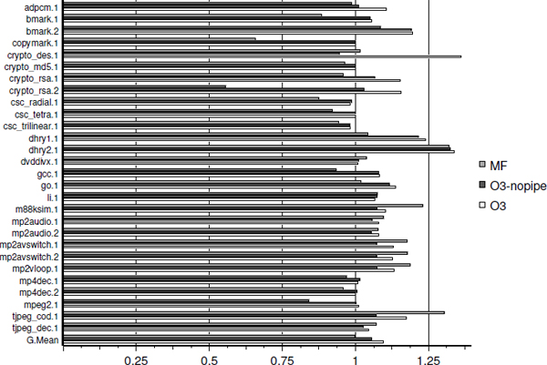
With the ST200 LAO disabled, the performances of the st200cc compiler at -03 and those of the multiflow-based compiler at -03 are equivalent, as the geometric mean entry for MF is almost 1 (last bars in Figure 4.6). However, on benchmarks like the tjpeg_coder, the multiflow-based compiler significantly outperforms the st200cc compiler, even with software pipelining. Investigations revealed that virtually all such st200cc performance problems are triggered by high register pressure on large basic blocks, where the prepass scheduling/register allocation/postpass scheduling approach of Open64 is unable to compete with the integrated register allocation and instruction scheduling of the multiflow-based compiler [LOW 93].

When accounting for the cache miss effects, the R3.2 st200cc compiler at optimization level -03 outperforms the multiflow-based compiler at optimization level -03 by 15% in cycles in geometric mean on the HP benchmarks, with the best case having an 18% higher performance and the worst case having a 5% lower performance. This is explained by the 12% geometric mean code size reduction of the st200cc compiler and its effective instruction cache optimizations [BID 04].

4.1.6. Time-indexed formulation of the modulo RCISP

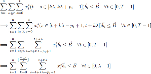
Based on the time-indexed formulation of the resource-constrained project scheduling problem (RCPSP) of Pritsker et al. [PRI 69] in section 3.3.1, the register-pressure equations of the modulo RPISP formulation of Eichenberger et al. [EIC 95b, EIC 97] in section 4.4.2 and the definition of the augmented dependence graph in section 4.1.1, we introduce a new time-indexed formulation for the modulo RCISP. This formulation is implemented in the ST200 LAO instruction scheduler as an experimental feature, as it requires linking with the commercial CPLEX package in order to solve the resulting integer linear programs.

The first extension of the RCPSP formulation needed for the modulo RCISP formulation is to account for the modulo resource constraints. In a modulo schedule, an operation O_i requires _i resources for the dates in [σ_i + kλ, σ_i + kλ + p_i – 1], k Δ (section 2.2.2). The resource requirement function _i(t) of O_i is written , so the inequalities [4.19] become:

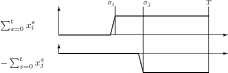
For the register pressure constraints, we consider the dependence graph augmented with the register lifetime nodes as defined in section 4.1.1. Let E_life denote the (i, j) pairs such that O_i is a producer node and O_j is its lifetime node. Let us also take advantage of the fact that most processors (in particular in the ST200 series) enable us to use and redefine a register at the same cycle and have a non-zero minimum register read after write (RAW) dependence latency. In such cases, it is correct to assume that a register lifetime extends from its definition date to its last use date minus one.

In the case = 0, the contribution to the register pressure at date t of the register produced by O_i and consumed by O_j is exactly the difference of two terms as illustrated in Figure 4.7. When > 0, the contribution to register pressure extends from date σ_i to date σ_j + λ. This yields the definition of by equalities [4.5]. In [4.6], we express the constraint that the register pressure at any date in the modulo schedule is not greater than the register availability R.

[4.5]

[4.6]

[4.7]

Figure 4.7. Definition of the contributions to the register pressure

To complete the modulo RCISP formulation, we minimize the schedule date of operation O_n+1, adapt the dependence inequalities [3.3] to the dependence latencies of – λ and eliminate the register pressure variables from [4.6], due to the equalities [4.5]. This yields:

[4.8]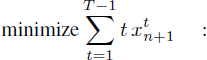

[4.9]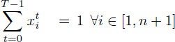

[4.10]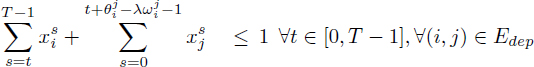

[4.11]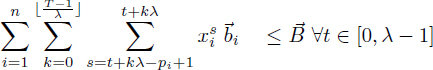

[4.12]

[4.13]

Here, we present some contributions to the field of instruction scheduling, in particular modulo scheduling:

To conclude, we anticipate that the techniques of machine scheduling will become increasingly relevant to VLIW instruction scheduling, in particular for the embedded computing applications. In such applications, high performances of the compiled applications enable the reduction of the system costs, whereas the compilation time is not really constrained. Embedded computing also yields instruction scheduling problems of significant size, especially for media processing.

Embedded computing thus motivates the development of advanced instruction scheduling techniques that deliver results close to optimality, rather than accepting the observed limitation of the traditional list-based instruction scheduling [COO 98, WIL 00]. An equally promising area of improvement of VLIW instruction scheduling is its full integration with the register allocation. In this area, the multiflow trace scheduling technology [LOW 93] is unchallenged.

Fortunately, modern embedded media processors, in particular VLIW processors such as the STMicroelectronics ST200 family, present a micro-architecture that allows for an accurate description using resources like in cumulative scheduling problems. This situation is all the more promising in cases of processors with clean pipelines like the ST200 family, as the resulting instruction scheduling problems only involve UET operations. Scheduling problems with cumulative resources and UET operations benefit from stronger machine scheduling relaxations, easier resource management in modulo scheduling and simpler time-indexed formulations.

With regards to the already compiler-friendly STMicroelectronics ST220 processor, the VLIW instruction scheduling problems it involves could be better solved if all its operation requirements on the cumulative resources were 0 or 1. This is mostly the case, except for the operations with immediate extensions, which require two issue slots (see Figure 2.1). Besides increasing the peak performances, removing this restriction enables the relaxation of the VLIW instruction scheduling problems into parallel machine scheduling problems with UET, problems which are optimally solved in polynomial time in several cases by the algorithm of Leung et al. [LEU 01].

4.2. Large neighborhood search for the resource-constrained modulo scheduling problem

The resource-constrained modulo scheduling problem (RCMSP) is motivated by the 1-periodic cyclic instruction scheduling problems that are solved by compilers when optimizing inner loops for instruction-level parallel processors. In production compilers, modulo schedules are computed by heuristics because even the most efficient integer programming formulation of resource-constrained modulo scheduling by Eichenberger and Davidson appears too expensive to solve relevant problems.

We present a new time-indexed integer programming formulation for the RCMSP and we propose a large neighborhood search heuristic to make it tractable. Based on experimental data from a production compiler, we show that this combination enables us to solve near-optimally RCMSPs of significant size. We also show that our large neighborhood search benefits to a lesser extent the resource-constrained modulo scheduling integer programming formulation of Eichenberger and Davidson.

Modulo scheduling is the cyclic instruction scheduling framework used by highly optimizing compilers to schedule instructions of innermost program loops [ALL 95]. Modulo scheduling is an effective optimization for instruction-level parallel processors [RAU 93a], especially the VLIW processors that are used for media processing in embedded devices such as set-top boxes, mobile phones, and DVD players. An example of a modern VLIW architecture is the Lx [FAR 00], which provides the basis of the successful STMicroelectronics ST200 VLIW processor family.

The modulo scheduling framework is distinguished by its focus on 1-periodic cyclic schedules with integral period, which leads to simplifications compared to the classic formulation of cyclic scheduling [HAN 95]. In the modulo scheduling framework, the period is called initiation interval and is the main indicator of the schedule quality. A RCMSP is a modulo scheduling problem where the resource constraints are adapted from the renewable resources of the RCPSP [BRU 99].

Optimal solutions to the RCMSP can be obtained by solving the classic integer programming formulations of Eichenberger and Davidson [EIC 97]. However, solving such a formulation is only tractable for modulo scheduling problems that comprise less than several tenth of operations³. While developing the ST200 production compiler at STMicroelectronics [DIN 04a], we found that modulo scheduling heuristics appeared to loosen effectiveness beyond such problem sizes, according to the lower bounds on the period obtained by relaxations.

To build high-quality modulo schedules for instruction scheduling problems of significant size, the contributions here are as follows: we show that for any assumed period λ, the RCMSP appears as a RCPSP with maximum time lags (RCPSP/max) and modulo resource constraints (section 4.3); we present a new time-indexed integer programming formulation for the RCMSP by adapting the time-indexed integer programming of Pritsker et al. [PRI 69] for the RCPSP/max (section 4.4); we propose a large neighborhood search (LNS) heuristic for the RCMSP, based on the adaptive reduction of margins and the resolution of the resulting time-indexed integer programming formulations by implicit enumeration (section 4.5).

4.3. Resource-constrained modulo scheduling problem

4.3.1. Resource-constrained cyclic scheduling problems

A basic cyclic scheduling problem [HAN 95] considers a set of generic operations {O_i }_1≤i≤n to be executed repeatedly, thus defining a set of operation instances , k ∈ . We call iteration k the set of operation instances . For any i ∈ [1, n] and k > 0 ∈ , let denote the schedule date of the operation instance Basic cyclic scheduling problems are constrained by uniform dependences, denoted as , where the latency and the distance are non-negative integers:

Figure 4.8. Sample cyclic instruction scheduling problem

In this section, we are focusing on resource-constrained cyclic scheduling problems, whose resource constraints are adapted from the RCPSPs [BRU 99]. Precisely, we assume a set of renewable resources, also known as cumulative resources, whose availabilities are given by an integral vector . Each generic operation O_i requires i resources for p_i consecutive units of time and this defines the resource requirements of all the operation instances . For the cyclic scheduling problems we consider, the cumulative use of the resources by the operation instances executing at any given time must not exceed .

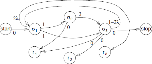
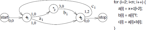
To illustrate the resource-constrained cyclic scheduling problems that arise from instruction scheduling, consider the inner loop source code and its dependence graph shown in Figure 4.8. To simplify the presentation, we did not include the memory access operations. Operation O₃ (c[i]=a[i]+b[i]) of iteration i must execute before operation O₁ (a[i]=x+c[i-2]) of iteration i+2 and this creates the uniform dependence with distance 2 between O₃ and O₁ (arc c_i in Figure 4.8). The dummy operations here labeled start and stop are introduced as source and sink of the dependence graph but have no resource requirements.

Assume that this code is compiled for a microprocessor whose resources are an adder and a multiplier. The adder and the multiplier may start a new operation every unit of time. However, due to pipelined implementation, the multiplier result is only available after three time units. This resource-constrained cyclic scheduling problem is defined by p₁ = p₂ = p₃ = 1, = (1, 1)^t, ₁ = ₃ = (0, 1)^t, ₂ = (1, 0)^t. The dependences are .

4.3.2. Resource-constrained modulo scheduling problem statement

A modulo scheduling problem is a cyclic scheduling problem where all operations have the same processing period λ ∆ , also called the initiation interval. Compared to cyclic scheduling problems, a main simplification is that modulo scheduling problems only need to consider the set of generic operations {O_i }_1≤i≤n. Precisely, by introducing the modulo schedule dates {σ_i}_1≤i≤n such that i ∆ [1, n], k > 0 : = σ_i + (k – 1)λ, the uniform dependence constraints become:

Let {σ_i}_1≤i≤n denote the modulo schedule dates of a set of generic operations {O_i}_1≤i≤n. An RCMSP is defined by [DIN 04a]:

– Uniform dependence constraints: for each such dependence , a valid modulo schedule satisfies σ_i + – ≤ σ_j. The dependence graph without the dependences whose > 0 is a directed acyclic graph (DAG);

– Modulo resource constraints: each operation O_i requires resources for all the time intervals [σ_i + kλ, σ_i + kλ + p_i – 1], k ∈ and the total resource use at any time cannot exceed a given availability . The integer value p_i is the processing time of O_i.

The primary objective of RCMSPs is to minimize the period λ. The secondary objective is usually to minimize the iteration makespan. In the contexts where the number of processor registers is a significant constraint, secondary objectives such as minimizing the cumulative register lifetimes [DIN 94] or the maximum register pressure [EIC 95b] are considered. This is not the case for the ST200 VLIW processors, so we will focus on makespan minimization.

4.3.3. Solving resource-constrained modulo scheduling problems

Most modulo scheduling problems cannot be solved by classic machine scheduling techniques, as the modulo resource constraints introduce operation resource requirements of unbounded extent. Also, the uniform dependence graph may include circuits (directed cycles), unlike machine scheduling precedence graphs that are acyclic. Even without the circuits, some modulo dependence latencies may also be negative. Thus, the RCMSP appears as a resource-constrained project scheduling problem with maximum time-lags (RCPSP/max) and modulo resource requirements.

In practice, building modulo schedules with heuristics is much easier than building RCPSP/max schedules. This is because the maximum time-lags of RCMSPs always include a term that is a negative factor of the period λ. Such constraints can always be made redundant by sufficiently increasing the period λ. A similar observation holds for the modulo resource constraints.

In the classic modulo scheduling framework [RAU 81, LAM 88a, RAU 96], a dichotomy search for the minimum λ that yields a feasible modulo schedule is performed, starting from with:

That is λ_rec is the minimum λ such that there are no positive length circuits in the dependence graph and λ_res is the minimum λ such that the renewable resources are not oversubscribed.

4.4. Time-indexed integer programming formulations

4.4.1. The non-preemptive time-indexed RCPSP formulation

We use the formulation previously defined in section 3.3.1:

[4.14]

[4.15]

[4.16]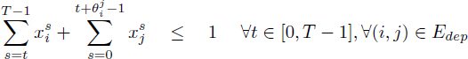

[4.17]

[4.18]

Equation [4.15] ensures that any operation is scheduled once. The inequalities [4.16] describe the dependence constraints, as proposed by Christofides et al. [CHR 87]. Given [4.15], inequalities [4.16] for any dependence (i, j) ∈ E_dep are equivalent to: and this implies σ_i < σ_j – . Finally, the inequalities [4.17] enforce the cumulative resource constraints for p_i ≥ 1. The extensions of the RCPSP with time-dependent resource availabilities (t) and resource requirements _i(t) are described in this formulation by generalizing [4.17] into [4.19]:

[4.19]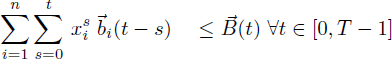

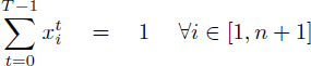
4.4.2. The classic modulo scheduling integer programming formulation

The classic integer programming formulation of the RCMSP is from Eichenberger and Davidson [EIC 97]. This formulation is based on a λ-decomposition of the modulo schedule dates, that is, i ∈ [0, n + 1] : σ_i = λϕ_i + τ_i, 0 ≤ τ_i < λ. Given an operation O_i, ϕ_i is its column number and τ_i is its row number. The formulation of Eichenberger and Davidson introduces the time-indexed variables for the row numbers, where if τ_i = t, otherwise . In particular, . The column numbers ϕ_i}_1≤i≤n are directly used in this formulation:

[4.20]

[4.21]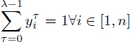

[4.22]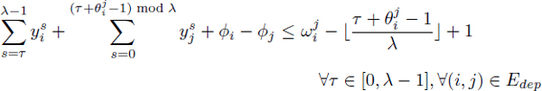

[4.23]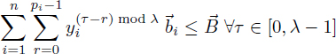

[4.24]

[4.25]

In this formulation, λ is assumed constant. Like in classic modulo scheduling, it is solved as the inner step of a dichotomy search for the minimum value of λ that allows a feasible modulo schedule.

4.4.3. A new time-indexed formulation for modulo scheduling

We propose a new time-indexed formulation for RCMSP, based on the time-indexed formulation of RCPSP/max of Pritsker et al. [PRI 69]. First, consider the modulo resource constraints. Each operation O_i requires _i resources for the dates in [σ_i + kλ, σ_i + kλ + p_i – 1], k ∈ (section 4.3.2). The resource requirement function _i(t) of O_i is written as ,; so [4.19] becomes:

To complete this new RCMSP formulation, we minimize the schedule date of operation O_n+1 and adapt the inequalities [4.16] to the modulo dependence latencies of – . This yields:

[4.26]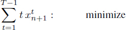

[4.27]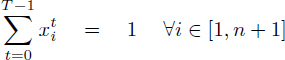

[4.28]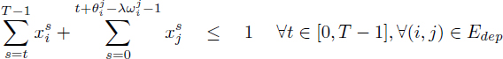

[4.29]

[4.30]

4.5. Large neighborhood search heuristic

4.5.1. Variables and constraints in time-indexed formulations

The time-indexed formulations for the RCMSP (and the RCPSP/max) involve variables and constraints in numbers that are directly related to any assumed earliest {e_i}_1≤i≤n and latest {1_i}_1≤i≤n schedule dates. Indeed, the number of variables is Most of the constraints are the dependence inequalities [4.28], and non-transitively redundant dependences appear to generate eT inequalities with . However, the first sum of [4.28] is 0 if t > l_i. Likewise, the second sum of [4.28] is 0 if t + – – 1 < e_j .So [4.28] is actually equivalent to:

[4.31]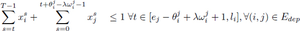

So [4.31] is redundant whenever e_j – + λ ≥ 1_i (e_j – ≥ 1_i in the case of the RCPSP/max).

The time-indexed formulation for the RCMSP (and the RCPSP/max) is therefore likely to become more tractable after reducing the possible schedule date ranges σ_i ∈ [e_i, 1_i]. The basic technique is to initialize e_i = r_i and 1_i = d_i – p_i, with {r_i}_1≤i≤n and {d_i}_1≤i≤n being the release dates and the due dates, and then propagate the dependence constraints using a label-correcting algorithm. More elaborate techniques have been proposed for the RCPSP [DEM 05]. Ultimately, all these margins reduction techniques rely on some effective upper bounding of the due dates {d_i}_1≤i≤n.

4.5.2. A large neighborhood search heuristic for modulo scheduling

In the case of the RCMSP, the primary objective is the period minimization. Heuristics build modulo schedules at some period λ that is often greater than the lower bound . When this happens, the feasibility of modulo scheduling at period λ – 1 is open. Moreover, it is not known how to bound the makespan at period λ – 1 given a makespan at period λ. This means that the effective upper bounding of the due dates in RCMSP instances is not available either.

To compensate for the lack of upper bounding, we propose an LNS for the RCMSP, based on adaptive margins reduction and implicit enumeration of the resulting time-indexed integer programs (using an mixed integer programming (MIP) solver). The LNS [SHA 98] is a metaheuristic where a large number of solutions in the neighborhood of an incumbent solution are searched by means of branch and bound, constraint programming or integer programming. The large neighborhood is obtained by fixing some variables of the incumbent solution while releasing others.

In the setting of time-indexed formulations, we consider as the neighborhood of an incumbent solution {σ_i}_1≤i≤n some schedule date ranges or margins {e_i, l_i : σ_i ∈ [e_i, l_i]}_1≤i≤n, which are made consistent under dependence constraint propagation. For each , we fix variables to zero and release variables . The fixed variables and the dependence constraints [4.31] found redundant given the margins are removed from the integer program.

We adapt the generic LNS algorithm of [PAL 04] by using margins to define the neighborhoods and by starting from a heuristic modulo schedule. The period λ is kept constant while this algorithm searches increasingly wider margins under a time budget in order to minimize the makespan. The key change is to replace the diversification operator of [PAL 04] by a decrement of the period to λ – 1 while keeping the schedule dates. This yields a pseudo-solution that may no longer be feasible due to the period change. Computational experience shows that a new solution at period λ – 1 can often be found in the neighborhood of this pseudo-solution, whenever the problem instance is feasible at period λ – 1. In case a solution at period λ – 1 is found, go back to minimize the makespan.

4.5.3. Experimental results with a production compiler

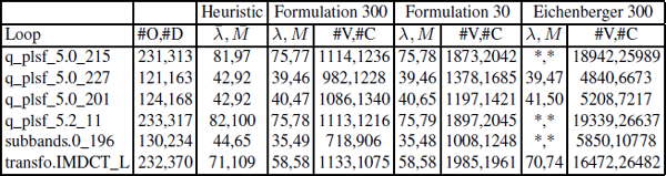
We implemented the two time-indexed formulations of RCMSP described in section 4.4 in the production compiler for the STMicroelectronics ST200 VLIW processor family [DIN 04a], along with the proposed LNS heuristic, then used the CPLEX 9.0 Callable Library to solve the resulting MIPs.

The table below reports experimental data for the largest loops that could not be solved with these formulations, assuming a timeout of 300 s and a time horizon of 4λ_min. Column #O,#D gives the number of operations and of non-redundant dependences. Column Heuristic λ, M displays the period and makespan computed by the ST200 production compiler insertion scheduling heuristic [DIN 04a]. The column groups Formulation 300, Formulation 30 and Eichenberger 300 correspond to the proposed LNS using our formulation and Eichenberger and Davidson’s formulation for timeout values of 300 s, 30 s and 300 s. In each group, column #V,#C gives the number or variables and constraints of the integer program sent to CPLEX 9.0. In all these cases, the Formulation LNS reached the λ_min.

4.6. Summary and conclusions

The RCMSP is a resource-constrained cyclic scheduling problem whose solutions must be 1-periodic of integral period λ. The primary minimization objective of the RCMSP is the period and the secondary objective is the makespan. Given any period λ, the RCMSP appears as a RCPSP/max and so-called modulo resource constraints.

Based on the RCPSP/max integer programming formulation of Pritsker et al. [PRI 69] and the strong dependence equations of Christofides et al. [CHR 87], we presented a new time-indexed integer programming formulation for the RCMSP. This formulation differs from the classic time-indexed integer programming formulation of the RCMSP by Eichenberger and Davidson [EIC 97].

Both formulations of the RCMSP are impractical to solve problems that comprise over several tenths of operations; so we propose a large LNS heuristic based on solving those integer programming formulations by implicit enumeration after adapting the operation margins. Experiments showed that this LNS heuristic is quite effective to find a solution at period λ – 1 given an incumbent solution at period λ, even for RCMSP instances that comprise hundreds of operations. To our knowledge, this is the first application of LNS to cyclic scheduling.

1 Although this term seems to imply EPIC architectures, J. Fisher in particular uses it for VLIW architectures.

2 This relation can be safely approximated by taking the lexical order of the operations in the program text.

3 An operation is an instance of an instruction in a program text. An instruction is a member of the processor instruction set architecture (ISA).