
12
Statistical Performance Analysis: The Speedup-Test Protocol
Numerous code optimization methods are usually experimented by doing multiple observations of the initial and the optimized execution times in order to declare a speedup. Even with a fixed input and execution environment, program execution times vary in general. Hence, different kinds of speedups may be reported: the speedup of the average execution time, the speedup of the minimal execution time, the speedup of the median, etc. Many published speedups in the literature are observations of a set of experiments. To improve the reproducibility of the experimental results, this chapter presents a rigorous statistical methodology regarding program performance analysis. We rely on well-known statistical tests (Shapiro–Wilk’s test, Fisher’s F-test, Student’s t-test, Kolmogorov–Smirnov test and Wilcoxon–Mann–Whitney test) to study whether the observed speedups are statistically significant or not. By fixing 0 < α < 1 a desired risk level, we are able to analyze the statistical significance of the average execution time as well as the median. We can also check if ![]() , the probability that an individual execution of the optimized code is faster than the individual execution of the initial code. Our methodology defines a consistent improvement compared to the usual performance analysis method in high-performance computing as in [JAI 91, LIL 00]. The Speedup-Test protocol certifying the observed speedups with rigorous statistics is implemented and distributed as an open-source tool based on R software in [TOU 10] and published in [TOU 13b].
, the probability that an individual execution of the optimized code is faster than the individual execution of the initial code. Our methodology defines a consistent improvement compared to the usual performance analysis method in high-performance computing as in [JAI 91, LIL 00]. The Speedup-Test protocol certifying the observed speedups with rigorous statistics is implemented and distributed as an open-source tool based on R software in [TOU 10] and published in [TOU 13b].
12.1. Code performance variation
The community of program optimization and analysis, code performance evaluation, parallelization and optimizing compilation has, for many decades, published numerous research and engineering articles in major conferences and journals. These articles study efficient algorithms, strategies and techniques to accelerate program execution times, or to optimize other performance metrics (MIPS, code size, energy/power, MFLOPS, etc.). The efficiency of a code optimization technique is generally published according to two principles, not necessarily disjoint. The first principle is to provide a mathematical proof given a theoretical model that the published research result is correct and/or efficient: this is the difficult part of research in computer science, since if the model is too simple, it would not represent the real world, and if the model is too close to the real world, the mathematics becomes too complex to digest. The second principle is to propose and implement a code optimization technique and to practice it on a set of chosen benchmarks in order to evaluate its efficiency. This chapter concerns the last point: how can we convince the community by rigorous statistics that the experimental study publishes fair and reproducible results.
Part of the non-reproducibility of the published experiments is explained by the fact that the observed speedups are sometimes “rare” events. It means that they are far from what we could observe if we redo the experiments multiple times. Even if we take an ideal situation where we use exactly the original experimental machines and software, it is sometimes difficult to reproduce exactly the same performance numbers again and again, experience after experience. Since some published performance numbers represent exceptional events, we believe that if a computer scientist succeeds in reproducing the performance numbers of his colleagues (with a reasonable error ratio), it would be equivalent to what rigorous probabilists and statisticians call a “surprise”. We argue that it is better to have a lower speedup that can be reproduced in practice than a rare speedup that can be remarked by accident.
One of the reasons for the non-reproducibility of the results is the variation of execution times of the same program given the same input and the same experimental environment. With the massive introduction of multi-core architectures, we observe that the variations of execution times become exacerbated because of the complex dynamic features influencing the execution: affinity and threads scheduling policy, synchronization barriers, resource sharing between threads, hardware mechanisms for speculative execution, etc. Consequently, if you execute a program (with a fixed input and environment) n times, it is possible to obtain n really distinct execution times. To illustrate this, we consider the experiments published in [MAZ 10]. We use the violin plot1 in Figure 12.1 to report the execution times of some SPEC OMP 2001 applications compiled with gcc. When we use thread-level parallelism (two or more threads), the execution time decreases overall but with a deep disparity. Consider, for instance, the case of swim. The version with two threads runs between 76 and 109 s, and the version with four threads runs between 71 and 90 s. This variability is also present when swim is compiled with icc (the Intel C compiler). The example of wupwise in Figure 12.1 is also interesting. The version with two threads runs between 376 and 408 s, and the version with six threads runs between 187 and 204 s. This disparity between the distinct execution times of the same program with the same data input cannot be justified by accidents or experimental hazards because we can observe that the execution times are not normally distributed and frequently have a bias.
Figure 12.1. Observed execution times of some SPEC OMP 2001 applications (compiled with gcc)

What makes a binary program execution time vary, even if we use the same data input, the same binary and the same execution environment? Here are some factors:
It is very difficult to control the complex combination of all the above influencing factors, especially on a supercomputer where the user is not allowed to have a root access to the machine. Consequently, if someone executes a program (with a fixed input and experimental environment) n times, it is possible to obtain n distinct execution times. The mistake is to assume that these variations are minor, and stable in general. The variations of execution times is something that we observe everyday, we cannot neglect them, but we can analyze them statistically with rigorous methodologies. Customary behavior in the community is to replace all the n execution times by a single value, such as the minimum, the mean, the median or the maximum, losing important data on variability and prohibiting the generation of statistics.
This chapter presents a rigorous statistical protocol to compare the performances of two code versions of the same application. While we consider that the performance of a program is measured by its execution time, our methodology is general and can be applied to other metrics of performance (energy consumption, for instance). It is important, however, to notice that our methodology applies for a continuous model of performance, not a discrete model. In a continuous model, we do not exclude integer values for measurements (that may be observed due to sampling), but we consider them as continuous data. We must also highlight that the name “Speedup-Test” does not rely on the usual meaning of statistical testing. Here, the term “test” in the “Speedup-Test” title is employed because our methodology makes intensive usage of proved statistical tests, and we do not define a new one.
This chapter is organized as follows: section 12.2 defines the background and notations needed for the chapter. Section 12.3 describes the core of our statistical methodology for the performance comparison between two code versions. Section 12.4 gives a quick overview on the free software we released for this purpose, called SpeedupTest. Section 12.5 shows how we can estimate the chance that the code optimization would provide a speedup on a program not belonging to the initial sample of benchmarks used for experiments. Section 12.6 describes some test cases and experiments using SpeedupTest. Section 12.7 discusses some related work before we conclude. In order to improve the fluidity and the readability of the chapter, we detail some notions in the appendix, making the chapter self-contained.
12.2. Background and notations
Let ![]() be an initial code, let
be an initial code, let ![]() ′ be a transformed version after applying the program optimization technique. Let I be a fixed data input for the programs
′ be a transformed version after applying the program optimization technique. Let I be a fixed data input for the programs ![]() and
and ![]() ′. If we execute the program
′. If we execute the program ![]() (I) n times, it is possible that we obtain n distinct execution times. Let X be the random variable representing the execution time of
(I) n times, it is possible that we obtain n distinct execution times. Let X be the random variable representing the execution time of ![]() (I). Let
(I). Let ![]() = {x1, …, xn} be a sample of observations of X, i.e the set of the observed execution times when executing
= {x1, …, xn} be a sample of observations of X, i.e the set of the observed execution times when executing ![]() (I) n times. The transformed code
(I) n times. The transformed code ![]() ′ can be executed m times with the same data input I producing m execution times too. Similarly, let Y be the random variable representing its execution time. Let
′ can be executed m times with the same data input I producing m execution times too. Similarly, let Y be the random variable representing its execution time. Let ![]() = {y1, …, ym} be a sample of observations of Y, it contains the m observed execution times of the code
= {y1, …, ym} be a sample of observations of Y, it contains the m observed execution times of the code ![]() ′(I).
′(I).
The theoretical means of X and Y are denoted as μX and μY, respectively. The theoretical medians of X and Y are denoted med(X) and med(Y). The theoretical variances are denoted as ![]() and
and ![]() . The cumulative distribution functions (CDF) are denoted FX(a) =
. The cumulative distribution functions (CDF) are denoted FX(a) = ![]() [X ≤ a] and FY(a) =
[X ≤ a] and FY(a) = ![]() [Y ≤ a], where
[Y ≤ a], where ![]() [X ≤ a] is the notation used for the probability that X ≤ a. The probability density functions are denoted as
[X ≤ a] is the notation used for the probability that X ≤ a. The probability density functions are denoted as ![]() and
and ![]() .
.
Since X and Y are two samples, their sample means are denoted as ![]() and
and ![]() , respectively. The sample variances are denoted as
, respectively. The sample variances are denoted as ![]() and
and ![]() . The sample medians of X and Y are denoted as
. The sample medians of X and Y are denoted as ![]() (X) and
(X) and ![]() (Y).
(Y).
After collecting X and Y (the sets of execution times of the codes ![]() (I) and
(I) and ![]() ′(I), respectively, for the same data input I), a simple definition of the speedup [HEN 02] sets it as
′(I), respectively, for the same data input I), a simple definition of the speedup [HEN 02] sets it as ![]() . In reality, since X and Y are random variables, the definition of a speedup becomes more complex. Ideally, we must analyze the probability density functions of X, Y and
. In reality, since X and Y are random variables, the definition of a speedup becomes more complex. Ideally, we must analyze the probability density functions of X, Y and ![]() to decide whether an observed speedup is statistically significant or not. Since this is not an easy problem, multiple types of observed speedups are usually reported in practice to simplify the performance analysis:
to decide whether an observed speedup is statistically significant or not. Since this is not an easy problem, multiple types of observed speedups are usually reported in practice to simplify the performance analysis:
1) The observed speedup of the minimal execution times:
![]()
2) The observed speedup of the mean (average) execution times:

3) The observed speedup of the median execution times:

Usually, the community publishes the best speedup among those observed, without any guarantee of reproducibility. In the below are our opinions on each of the above speedups:
– Regarding the observed speedup of the minimal execution times, we do not advise its use for many reasons. Appendix A of [TOU 10] explains why using the observed minimal execution time is not a fair choice regarding the chance of reproducing the result.
– Regarding the observed speedup of the mean execution time, it is well understood in statistical analysis but remains sensitive to outliers. Consequently, if the program under optimization study is executed a few times by an external user, the latter may not be able to observe the reported average. However, the average execution time is commonly accepted in practice.
– Regarding the observed speedup of the median execution times, it is the one that is used by the SPEC organization [STA 06]. Indeed, the median is a better choice for reporting speedups, because the median is less sensitive to outliers. Furthermore, some practical cases show that the distribution of the execution times are skewed, making the median a better candidate for summarizing the execution times into a single number.
The previous speedups are defined for a single application with a fixed data input ![]() (I). When multiple benchmarks are tested, we are sometimes faced with the need of reporting an overall speedup for the whole set of benchmarks. Since each benchmark may be very different from the other or may be of distinct importance, sometimes a weight W(
(I). When multiple benchmarks are tested, we are sometimes faced with the need of reporting an overall speedup for the whole set of benchmarks. Since each benchmark may be very different from the other or may be of distinct importance, sometimes a weight W(![]() j) is associated with a benchmark
j) is associated with a benchmark ![]() j. After running and measuring the speed of every benchmark (with multiple runs of the same benchmark), we define ExecutionTime(
j. After running and measuring the speed of every benchmark (with multiple runs of the same benchmark), we define ExecutionTime(![]() j, Ij) as the considered execution time of the code
j, Ij) as the considered execution time of the code ![]() j having Ij as data input. ExecutionTime(
j having Ij as data input. ExecutionTime(![]() j, Ij) replaces all the observed execution times of
j, Ij) replaces all the observed execution times of ![]() j(Ij) with one of the usual functions (mean, median and minimal), i.e. the mean or the median or the minimal of the observed execution times of the code
j(Ij) with one of the usual functions (mean, median and minimal), i.e. the mean or the median or the minimal of the observed execution times of the code ![]() j. The overall observed speedup of a set of b benchmarks is defined by the following equation:
j. The overall observed speedup of a set of b benchmarks is defined by the following equation:
[12.1] 
This speedup is a global measure of the acceleration of the execution time. Alternatively, some users prefer to consider G the overall gain, which is a global measure of how much (in percentage) the overall execution time has been reduced:
[12.2] 
Depending on which function has been used to compute ExecutionTime(![]() j , Ij), we speak about the overall speedup and gain of the average execution time, median execution time or minimal observed execution time.
j , Ij), we speak about the overall speedup and gain of the average execution time, median execution time or minimal observed execution time.
All the above speedups are observation metrics based on samples that do not guarantee their reproducibility since we are not sure about their statistical significance. Section 12.3 studies the question for the average and median execution times. Studying the statistical significance of the speedup of the minimal execution time remains a difficult open problem in non-parametric statistical theory (unless the probability density function is known, which is not the case in practice).
12.3. Analyzing the statistical significance of the observed speedups
The observed speedups are performance numbers observed once (or multiple times) on a sample of executions. Does this mean that other executions would conclude with similar speedups? How can we be sure about this question if no mathematical proof exists, and with which confidence level? This section answers this question and shows that we can test if μX > μY and if med(X) > med(Y). For the remainder of this section, we define 0 < α < 1 as the risk (probability) of error, which is the probability of announcing a speedup that does not really exist (even if it is observed on a sample). Conversely, (1 – α) is the usual confidence level. Usually, α is a small value (for instance, α = 5%).
The reader must be aware that in statistics, the risk of error is included in the model; therefore, we are not always able to decide between two contradictory situations (contrary to logic where a quantity cannot be true and false at the same time). Furthermore, the misuse of language defines (1 – α) as a confidence level, while this is not exactly true in the mathematical sense. Indeed, there are two types of risks when we use statistical tests; Appendix A7.2 describes these two risks and discusses the notion of the confidence level. We often say that a statistical test (normality test, Student’s test, etc.) concludes favorably by a confidence level (1 – α) because it did not succeed in rejecting the tested hypothesis with a risk level equal to α. When a statistical test does not reject a hypothesis with a risk equal to α, there is usually no proof that the contrary is true with a confidence level of (1 – α). This way of reasoning is admitted for all statistical tests since in practice it works well.
12.3.1. The speedup of the observed average execution time
Having two samples ![]() and
and ![]() , deciding if μX the theoretical mean of X is higher than μY, the theoretical mean of Y with a confidence level 1 – α can be done due to the Student’s t-test [JAI 91]. In our situation, we use the one-sided version of the Student’s t-test and not the two-sided version (since we want to check whether the mean of X is greater than the mean of Y, not to test if they are simply distinct). Furthermore, the observation xi ∈
, deciding if μX the theoretical mean of X is higher than μY, the theoretical mean of Y with a confidence level 1 – α can be done due to the Student’s t-test [JAI 91]. In our situation, we use the one-sided version of the Student’s t-test and not the two-sided version (since we want to check whether the mean of X is greater than the mean of Y, not to test if they are simply distinct). Furthermore, the observation xi ∈ ![]() does not correspond to another observation yj ∈
does not correspond to another observation yj ∈ ![]() ; so we use the unpaired version of the Student’s t-test.
; so we use the unpaired version of the Student’s t-test.
12.3.1.1. Remark on the normality of the distributions of X and Y
The mathematical proof of the Student’s t-test is valid for Gaussian distributions only [SAP 90, BRO 02]. If X and Y are not from Gaussian distributions (normal is synonymous to Gaussian), then the Student’s t-test is known to stay robust for large samples (due to the central limit theorem), but the computed risk α is not exact [BRO 02, SAP 90]. If X and Y are not normally distributed and are small samples, then we cannot conclude with the Student’s t-test.
12.3.1.2. Remark on the variances of the distributions of X and Y
In addition to the Gaussian nature of X and Y, the original Student’s t-test was proved for populations with the same variance (![]() ≈
≈ ![]() ). Consequently, we also need to check whether the two populations X and Y have the same variance by using the Fisher’s F-test, for instance. If the Fisher’s F-test concludes that
). Consequently, we also need to check whether the two populations X and Y have the same variance by using the Fisher’s F-test, for instance. If the Fisher’s F-test concludes that ![]() ≠
≠ ![]() , then we must use a variant of Student’s t-test that considers Welch’s approximation of the degree of freedom.
, then we must use a variant of Student’s t-test that considers Welch’s approximation of the degree of freedom.
12.3.1.3. The size needed for the samples X and Y
The question now is to know what is a large sample. Indeed, this question is complex and cannot be answered easily. In [LIL 00, JAI 91], a sample is said to be large when its size exceeds 30. However, that size is well known to be arbitrary, it is commonly used for a numerical simplification of the test of Student2. Note that n > 30 is not a size limit needed to guarantee the robustness of the Student’s t-test when the distribution of the population is not Gaussian, since the t-test remains sensitive to outliers in the sample. Appendix C in [TOU 10] gives a discussion on the notion of large sample. In order to set the ideas, let us consider that n > 30 defines the size of large samples: some books devoted to practice [LIL 00, JAI 91] write a limit of 30 between small (n ≤ 30) and large (n > 30) samples.
12.3.1.4. Using the Student’s t-test correctly
H0, the null hypothesis that we try to reject (in order to declare a speedup) by using Student’s t-test, is that μX ≤ μY, with an error probability (of rejecting H0 when H0 is true, i.e. when there is no speedup) equal to α. If the test rejects this null hypothesis, then we can accept Hα the alternative hypothesis μX > μY with a confidence level 1 – α (Appendix A7.2 explains the exact meaning of the term confidence level). The Student’s t-test computes a p-value, which is the smallest probability of error to reject the null hypothesis. If p-value≤ α, then the Student’s t-test rejects H0 with a risk level lower than α. Hence, we can accept Ha with a confidence level (1 – α). Appendix A7.2 gives more details on hypothesis testing in statistics, and on the exact meaning of the confidence level.
As explained before, the correct usage of the Student’s t-test is conditioned by:
The detailed description of the Speedup-Test protocol for the average execution time is illustrated in Figure 12.2.
The problem with the average execution time is its sensibility to outliers. Furthermore, the average is not always a good indicator of the observed execution time felt by the user. In addition, the Student’s test has been proved only for Gaussian distributions, while it is rare in practice to observe them for program execution times [MAZ 10]: the usage of the Student’s t-test for non-Gaussian distributions is admitted for large samples but the risk level is no longer guaranteed.
The median is generally preferable to the average for summarizing the data into a single number. The next section shows how to check if the speedup of the median is statistically significant.
12.3.2. The speedup of the observed median execution time, as well as individual runs
This section presents the Wilcoxon–Mann–Whitney [HOL 73] test, a robust statistical test to check whether the median execution time has been reduced or not after a program transformation. In addition, the statistical test we are presenting also checks whether ![]() [X > Y] > 1/2, as is proved in Appendix D of [TOU 10, p. 35]: this is a very good information for the real speedup felt by the user (
[X > Y] > 1/2, as is proved in Appendix D of [TOU 10, p. 35]: this is a very good information for the real speedup felt by the user (![]() [X > Y] > 1/2 means that there is more chance that a single random run of the optimized program will be faster than a single random run of the initial program).
[X > Y] > 1/2 means that there is more chance that a single random run of the optimized program will be faster than a single random run of the initial program).
Figure 12.2. The Speedup-Test protocol for analyzing the average execution time

Contrary to the Student’s t-test, the Wilcoxon–Mann–Whitney test does not assume any specific distribution for X and Y. The mathematical model [HOL 73, p. 70] imposes that the distributions of X and Y differ only by a location shift Δ; in other words, that
![]()
Under this model (known as the location model), the location shift equals Δ = med(X)–med(Y) (as well as Δ = μX–μY in fact) and X and Y consequently do not differ in dispersion. If this constraint is not satisfied, then as admitted for the Student’s t-test, the Wilcoxon–Mann–Whitney test can still be used for large samples in practice but the announced risk level may not be preserved. However, two advantages of this model is that the normality is no longer needed and that assumptions on the sign of Δ can be readily interpreted in terms of ![]() [X > Y].
[X > Y].
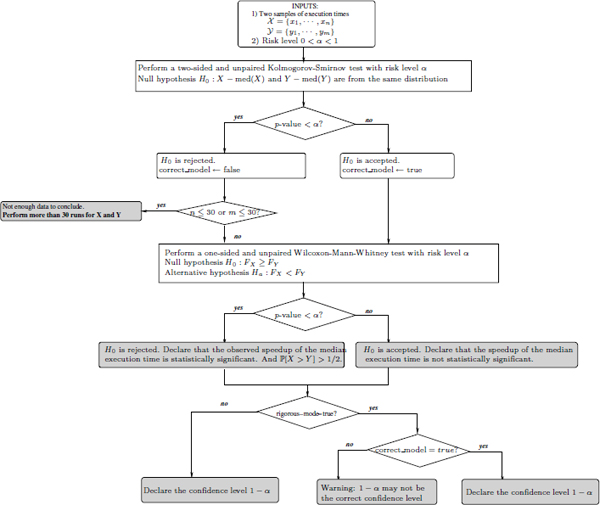
To check if X and Y satisfy the mathematical model of the Wilcoxon–Mann–Whitney test, a possibility is to use Kolmogorov–Smirnov’s two-sample test [CON 71] as described below.
12.3.2.1. Using the test of Kolmogorov–Smirnov at first step
The objective is to test the null hypothesis H0 of the equality of the distributions of the variables X – med(X) and Y – med(Y), using the Kolmogorov–Smirnov’s two-sample test applied to the observations xi – ![]() (X) and yj –
(X) and yj – ![]() (Y). The Kolmogorov–Smirnov test computes a p-value: if p-value ≤ α, then H0 is rejected with a risk level α. That is, X and Y do not satisfy the mathematical model needed by the Wilcoxon–Mann–Whitney test. However, as said before, we can still use the test in practice for sufficiently large samples but the risk level may not be preserved [HOL 73].
(Y). The Kolmogorov–Smirnov test computes a p-value: if p-value ≤ α, then H0 is rejected with a risk level α. That is, X and Y do not satisfy the mathematical model needed by the Wilcoxon–Mann–Whitney test. However, as said before, we can still use the test in practice for sufficiently large samples but the risk level may not be preserved [HOL 73].
12.3.2.2. Using the test of Wilcoxon–Mann–Whitney
As done previously with the Student’s t-test for comparing between two averages, here we want to check whether the median of X is greater than the median of Y, and if ![]() [X > Y] >
[X > Y] > ![]() . This requires us to use the one-sided variant of the Wilcoxon–Manny–Whitney test. In addition, since the observation xi from X does not correspond to an observation yj from Y, we use the unpaired version of the test.
. This requires us to use the one-sided variant of the Wilcoxon–Manny–Whitney test. In addition, since the observation xi from X does not correspond to an observation yj from Y, we use the unpaired version of the test.
We set the null hypothesis H0 of Wilcoxon–Mann–Whitney test as FX ≥ FY, and the alternative hypothesis as Ha : FX < FY. As a matter of fact, the (functional) inequality FX < FY means that X tends to be greater than Y. In addition, note that under the location shift model, Ha is equivalent to the fact that the location shift Δ is > 0.
The Wilcoxon–Mann–Whitney test computes a p-value. If the p-value ≤ α, then H0 is rejected. That is, we admit Ha with a confidence level 1 – α: FX > FY. This leads us to declare that the observed speedup of the median execution times is statistically significant, med(X) > med(Y) with a confidence level 1 – α, and ![]() [X > Y] >
[X > Y] > ![]() . If the null hypothesis is not rejected, then the observed speedup of the median is not considered to be statistically significant.
. If the null hypothesis is not rejected, then the observed speedup of the median is not considered to be statistically significant.
Figure 12.3 illustrates the speedup-test protocol for the median execution time.
Figure 12.3. The Speedup-Test protocol for analyzing the median execution time
12.4. The Speedup-Test software
The performance evaluation methodology described in this chapter has been implemented and automated in a software called SpeedupTest. It is a command line software that works on the shell: the user specifies a configuration file, then the software reads the data, checks if the observed speedups are statistically significant and prints full reports. SpeedupTest is based on R [TEA 08]; it is available as a free software in [TOU 10]. The programming language is a script (R and bash), so the code itself is portable across multiple operating systems and hardware platforms. We have tested it successfully on Linux, Unix and Mac OS environments (other platforms may be used).
The input of the software is composed of:
– A unique configuration file in CSV format: it contains one line per benchmark under study. For each benchmark, the user has to specify the file name of the initial set of performance observations (![]() sample) and the optimized performances (
sample) and the optimized performances (![]() sample). Optionally, a weight (W(
sample). Optionally, a weight (W(![]() )) and a confidence level can be defined individually per benchmark or globally for all benchmarks. It is possible to ask SpeedupTest to compute the highest confidence level per benchmark to declare statistical significance of speedups.
)) and a confidence level can be defined individually per benchmark or globally for all benchmarks. It is possible to ask SpeedupTest to compute the highest confidence level per benchmark to declare statistical significance of speedups.
– For each benchmark (two code versions), the observed performance data collected needs to be saved in two distinct raw text files: a file for the ![]() sample and another for the
sample and another for the ![]() sample.
sample.
The reason why we split the input into multiple files is to simplify the configuration of data analysis. Due to our choice, making multiple performance comparisons requires modifications in the CSV configuration file only, and the input data files remain unchanged.
SpeedupTest accepts some optional parameters in the command line, such as a global confidence level (to be applied to all benchmarks), weights to be applied on benchmarks and required precision for confidence intervals (not detailed in this chapter but explained in [TOU 10]).
The output of the software is composed of four distinct files:
1) a global report that prints the overall speedups and gains of all the benchmarks;
2) a file that details the individual speedup per benchmark, its confidence level and its statistical significance;
3) a warning file that explains for some benchmarks why the observed speedup is not statistically significant;
4) an error file that prints any misbehavior of the software (for debugging purposes).
The user manual of the software, sample data and demos are present in [TOU 10]. The next section presents an experimental use of the software and studies the probability of getting a significant statistical speedup on any program that does not necessarily belong to the initial set of tested benchmarks.
12.5. Evaluating the proportion of accelerated benchmarks by a confidence interval
Computing the overall performance gain or speedup for a sample of b programs does not allow us to estimate the quality or the efficiency of the code optimization technique. In fact, within the b programs, only a fraction of a benchmarks have a speedup, and b – a programs have a slowdown. In this section, we want to analyze the probability p to get a statistically significant speedup if we apply a code transformation. If we consider a sample of b programs only, we could say that the chance to observe a speedup is ![]() . But this computed chance
. But this computed chance ![]() is observed on a sample of b programs only. So what is the confidence interval of p? The following paragraphs answer this question.
is observed on a sample of b programs only. So what is the confidence interval of p? The following paragraphs answer this question.
In probability theory, we can study the random event {the program is accelerated with the code optimization under study}. This event has two possible values: true or false, so it can be represented by a Bernoulli variable. To compile accurate statistics, it is very important that the initial set of b benchmarks be selected randomly from a large database of representative benchmarks. If the set of b benchmarks are selected manually and not randomly, then there is a bias in the sample and the statistics we compute in this section are wrong. For instance, if the set of b programs are retrieved from well-known benchmarks (SPEC or others), then they cannot be considered as sufficiently random, because well-known benchmarks have been selected manually by a group of people, not selected randomly from a large database of programs.
If we randomly select a sample of b representative programs as a sample of benchmarks, we can measure the chance of getting the fraction of accelerated programs as ![]() . The higher this proportion is, the better the quality of the code optimization would be. In fact, we want to evaluate whether the code optimization technique is beneficial for a large fraction of programs. The proportion C =
. The higher this proportion is, the better the quality of the code optimization would be. In fact, we want to evaluate whether the code optimization technique is beneficial for a large fraction of programs. The proportion C = ![]() has only been observed on a sample of b programs. There are many techniques for estimating the confidence interval for p (with a risk level α).
has only been observed on a sample of b programs. There are many techniques for estimating the confidence interval for p (with a risk level α).
The simplest and most commonly used formula relies on approximating the binomial distribution with a normal distribution. In this situation, the confidence interval is given by the equation C ![]() r, where
r, where

In other words, the confidence interval of the proportion is equal to [C – r, C + r]. Here, z1–α/2 represents the value of the quartile of order 1 – α/2 of the standard normal distribution (![]() [N(0,1) > z] =
[N(0,1) > z] = ![]() ). This value is available in a known precomputed table and in many softwares (Table A.2 in [JAI 91]). We should notice that the previous formula of the confidence interval of the proportion
). This value is available in a known precomputed table and in many softwares (Table A.2 in [JAI 91]). We should notice that the previous formula of the confidence interval of the proportion ![]() is accurate only when the value of
is accurate only when the value of ![]() are not too close from 0 or 1. A frequently cited rule of thumb is that the normal approximation works well as long as
are not too close from 0 or 1. A frequently cited rule of thumb is that the normal approximation works well as long as ![]() , as indicated, for instance, in [SAP 90] (section 2.7.2). However, in another contribution [BRO 01], that condition was discussed and criticized. The general subject of choosing appropriate sample size, which ensures an accurate normal approximation, was discussed in Chapter VII 4, example (h) of the reference book [FEL 68].
, as indicated, for instance, in [SAP 90] (section 2.7.2). However, in another contribution [BRO 01], that condition was discussed and criticized. The general subject of choosing appropriate sample size, which ensures an accurate normal approximation, was discussed in Chapter VII 4, example (h) of the reference book [FEL 68].
When the approximation of the binomial distribution with a normal one is not accurate, other techniques may be used, which will not be presented here. The R software has an implemented function that computes the confidence interval of a proportion based on the normal approximation of a binomial distribution, see the example below.
EXAMPLE (WITH R) 12.1.– Having b = 30 benchmarks selected randomly from a large set of representative benchmarks, we obtained a speedup on only a = 17 cases. We want to compute the confidence interval for p around the proportion C=17/30=0.5666 with a risk level equal to α = 0.1 = 10%. We easily estimate the confidence interval of C using the R software as follows:

Since ![]() , the computed confidence interval of the proportion is accurate. Note that this confidence interval is invalid if the initial set of b = 30 benchmarks was not randomly selected among a large number of representative benchmarks.
, the computed confidence interval of the proportion is accurate. Note that this confidence interval is invalid if the initial set of b = 30 benchmarks was not randomly selected among a large number of representative benchmarks.
The above test allows us to say that we have a 90% chance that the proportion of accelerated programs is between 40.27% and 71.87%. If this interval is too wide for the purpose of the study, we can reduce the confidence level as an initial, and straightforward, solution. For instance, if I consider α = 50%, the confidence interval of the proportion becomes [49.84%, 64.23%].
The next formula [JAI 91] gives the minimal number b of benchmarks to be selected randomly if we want to estimate the proportion confidence interval with a precision equal to r% with a risk level α:
![]()
EXAMPLE (WITH R) 12.2.– In the previous example, we obtained an initial proportion equal to C = 17/30 = 0.5666. If we want to estimate the confidence interval with a precision equal to 5% with a risk level of 5%, we put r = 0.05 and we read in the quartiles tables z1–0.05/2 = z0.975 = 1.960. The minimal number of benchmarks to observe is then equal to: ![]() . We need to randomly select 378 benchmarks in order to assert that we have a 95% chance that the proportions of accelerated programs are in the interval 0.566
. We need to randomly select 378 benchmarks in order to assert that we have a 95% chance that the proportions of accelerated programs are in the interval 0.566 ![]() 5%.
5%.
The following section presents our implementation of the performance evaluation methodology.
12.6. Experiments and applications
Let us first describe the set of program benchmarks; their source codes are written in C and Fortran:
1) SPEC CPU 2006: a set of 17 sequential applications. They are executed using the standard ref data input.
2) SPEC OMP 2001: a set of 9 parallel OpenMP applications. Each application can be run in a sequential mode, or in a parallel mode with 1, 2, 4, 6 or 8 threads, respectively. They are executed using the standard train data input.
From our experience, we consider that all the benchmarks have equal weight (∀k, W(![]() k) = 1). The binaries of the above benchmarks have been generated using two distinct compilers of equivalent release date: gcc 4.1.3 and Intel icc 11.0. These compiler versions were the ones available when our experimental studies were carried out. Newer compiler versions may be available now and in the future. Other compilers may be used. A typical future project would be to make a fair performance comparison between multiple parallelizing compilers. Note that our experiments have no influence on the statistical methodology that we describe, since we base our work on mathematics, but not on experimental performance data. Any performance data can be analyzed, and the versions of the tools that are used to log performance data have no influence on the theory behind them.
k) = 1). The binaries of the above benchmarks have been generated using two distinct compilers of equivalent release date: gcc 4.1.3 and Intel icc 11.0. These compiler versions were the ones available when our experimental studies were carried out. Newer compiler versions may be available now and in the future. Other compilers may be used. A typical future project would be to make a fair performance comparison between multiple parallelizing compilers. Note that our experiments have no influence on the statistical methodology that we describe, since we base our work on mathematics, but not on experimental performance data. Any performance data can be analyzed, and the versions of the tools that are used to log performance data have no influence on the theory behind them.
We experimented multiple levels (compiler flags and options) of code optimizations carried out by both compilers. Our experiments were conducted on a Linux workstation (Intel Core 2, two quad-core Xeon processors, 2.33 GHz.). For each binary version, we repeated the execution of the benchmark 31 times and recorded the measurement. For a complete description of the experimental setup and environment used to collect the performance data, please refer to [MAZ 10]. The data are released publicly in [TOU 10]. This section focuses more on data analysis than data collection techniques. Next, we describe three possible applications of the SpeedupTest software. Note that applying the SpeedupTest in every section below requires less than 2 s of computation on a MacBook pro (2.53 GHz Intel Core 2 Duo).
The following section provides an initial set of experiments that compare the performances of different compiler flags.
12.6.1. Comparing the performances of compiler optimization levels
We consider the set of SPEC CPU 2006 (17 programs). Every source code is compiled using gcc 4.1.3 with three compiler optimization flags: –O0 (no optimization), –O1 (basic optimizations) and –O3 (aggressive optimizations). That is, we generate three different binaries per benchmark. We want to test whether the optimization levels –O1 and –O3 are really efficient compared to –O0. This requires us to consider 34 couples of comparisons: for every benchmark, we compare the performance of the binary generated by –O1 versus –O0 and the one generated by –O3 versus –O0.
The observed performances of the benchmarks reported by the tool are:
Overall gain (ExecutionTime=mean) = 0.464
Overall speedup (ExecutionTime=mean) = 1.865
Overall gain (ExecutionTime=median) = 0.464
Overall speedup (ExecutionTime=median) = 1.865
The overall observed gain and speedups are identical here because in this set of experiments, the observed median and mean execution times of every benchmark were almost identical (with three digits of precision). Such observations advocate that the binaries generated due to optimization levels –O1 and –03 are really efficient compared to –O0. To be confident of such a conclusion, we need to rely on the statistical significance of the individual speedups per benchmark (for both median and average execution times). They have all been accepted with a confidence level equal to 95%, i.e. with a risk level of 5%. Our conclusions remain the same even if we reduce the confidence level to 1%, i.e. with a risk level of 99%.
The tool also computes the following information:
The observed proportion of accelerated benchmarks (speedup of the mean) a/b = 34/34 = 1 The confidence level for computing proportion confidence interval is 0.9. Proportion confidence interval (speedup of the mean) = [0.901; 1] Warning: this confidence interval of the proportion may not be accurate because the validity condition {a(1-a/b)>5} is not satisfied.
Here, the tool states that the probability that the compiler optimization option –03 would produce a speedup (versus –O1) of the mean execution time belongs to the interval [0.901; 1]. However, as noted by the tool, this confidence interval may not be accurate because the validity condition ![]() is not satisfied. Recall that the computed confidence interval of the proportion is invalid if b the experimented set of benchmarks is not randomly selected among a huge number of representative benchmarks. Since we experimented selected benchmarks from SPEC CPU 2006, this condition is not satisfied; so we cannot advocate for the precision of the confidence interval.
is not satisfied. Recall that the computed confidence interval of the proportion is invalid if b the experimented set of benchmarks is not randomly selected among a huge number of representative benchmarks. Since we experimented selected benchmarks from SPEC CPU 2006, this condition is not satisfied; so we cannot advocate for the precision of the confidence interval.
Instead of analyzing the speedups obtained by compiler flags, one could obtain speedups by launching parallel threads. The next section studies this aspect.
12.6.2. Testing the performances of parallel executions of OpenMP applications
In this section, we investigate the efficiency of a parallel execution against a sequential application. We consider the set of 9 SPEC OMP 2001 applications. Every application is executed with 1, 2, 4, 6 and 8 threads, respectively. We compare every version to the sequential code (no threads). The binaries have been generated with the Intel icc 11.0 compiler using the flag –03. So we have to conduct a comparison between 45 couples of benchmarks.
The observed performances of the benchmarks reported by the tool are:
Overall gain (ExecutionTime=mean) = 0.441
Overall speedup (ExecutionTime=mean) = 1.79
Overall gain (ExecutionTime=median) = 0.443
Overall speedup (ExecutionTime=median) = 1.797
These overall performance metrics clearly advocate that a parallel execution of the application is faster than a sequential execution. However, by analyzing the statistical significance of the individual speedups with a risk level of 5%, we find that:
– As expected, none of the single-threaded versions of the code were faster than the sequential version: this is because a sequential version has no thread overhead, and the compiler is better able to optimize the sequential code compared to the singlethreaded code.
– Strange enough, the speedup of the average and median execution times has been rejected in five cases (with two threads or more). In other words, the parallel version of the code in five cases is not faster (in average and median) than the sequential code.
Our conclusions remain the same if we increase the risk level to 20% or if we use the gcc 4.1.3 compiler instead of icc 11.0.
The tool also computes the following information:
The observed proportion of accelerated benchmarks (speedup of the mean) a/b = 31/45 = 0.689 The confidence level for computing proportion confidence interval is 0.95. Proportion confidence interval (speedup of the mean) = [0.532; 0.814] The minimal needed number of randomly selected benchmarks is 330 (in order to have a precision r=0.05).
Here the tool indicates that:
1) The probability that a parallel version of an OpenMP application would produce a speedup (of the average execution time) against the sequential version belongs to the interval [0.532; 0.814].
2) If this probability confidence interval is not tight enough, and if the user requires a confidence interval with a precision of r = 5%, then the user has to make experiments on a minimal number of randomly selected benchmarks b = 330.
Let us now make a statistical comparison between the program performance obtained by two distinct compilers. That is, we want to check whether the icc 11.0 produces more efficient codes compared to gcc 4.1.3.
12.6.3. Comparing the efficiency of two compilers
In this last section of performance evaluation, we want to answer the following question: which compiler (gcc 4.1.3 or Intel icc 11.0) is the best on an Intel Dell workstation? Both compilers have similar release dates and both are tested with aggressive code optimization level –O3.
A compiler or a computer architecture expert would say, clearly, that the Intel icc 11.0 compiler would generate faster codes. The reason for this is that gcc 4.1.3 is a free general purpose compiler that is designed for almost all processor architectures, while icc 11.0 is a commercial compiler designed for Intel processors only: the code optimizations of icc 11.0 are specially focused for the workstation on which the experiments have been conducted, while gcc 4.1.3 has less focus on Intel processors.
The experiments have been conducted using the set of nine SPEC OMP 2001 applications. Every application is executed in a sequential mode (without thread), or in parallel mode (with 1, 2, 4, 6 and 8 threads, respectively). We compare the performances of the binaries generated by icc 11.0 with the binaries generated by gcc 4.1.3. So, we make a comparison between 54 couples.
The observed performances of the benchmarks reported by the tool are:
Overall gain (ExecutionTime=mean) = 0.14
Overall speedup (ExecutionTime=mean) = 1.162
Overall gain (ExecutionTime=median) = 0.137
Overall speedup (ExecutionTime=median) = 1.158
These overall performance metrics clearly advocate that icc 11.0 generated faster codes than gcc 4.1.3. However, by analyzing the statistical significance of the individual speedups, we find that:
– With a risk level of 5%, the speedup of the average execution time is rejected in 14 cases among 54. If the risk is increased to 20%, the number of rejections decreases to 13 cases. With a risk of 99%, the number of rejections decreases to 11 cases.
– With a risk level of 5%, the speedup of the median execution time is rejected in 13 cases among 54. If the risk is increased to 20%, the number of rejections decreases to 12 cases. With a risk of 99%, the number of rejections remains at 12 cases among 54.
Here we can conclude that the efficiency of the gcc 4.1.3 compiler is not as bad as thought, however is still under the level of efficiency for a commercial compiler such as icc 11.0.
The tool also computes the following information:
The observed proportion of accelerated benchmarks (speedup of the median) a/b = 41/54 = 0.759. The confidence level for computing proportion confidence interval is 0.95. Proportion confidence interval (speedup of the median) = [0.621; 0.861]. The minimal number of randomly selected benchmarks needed is 281 (in order to have a precision r = 0.05).
Here the tool says that:
1) The probability that icc 11.0 beats gcc 4.1.3 (produces a speedup of the median execution time) on a randomly selected benchmark belongs to the interval [0.621; 0.861].
2) If this probability confidence interval is not tight enough, and if the user requires a confidence interval with a precision of r = 5%, then the user has to make experiments on a minimal number of randomly selected benchmarks b = 281!
12.6.4. The impact of the Speedup-Test protocol over some observed speedups
In this section, we give a synthesis of our experimental data to show that some observed speedups (that we call “hand made”) are not statistically significant. In each benchmark family, we counted the number of non-statistically significant speedups among those that are “hand made”. Table 12.1 gives a synthesis. The first column describes the benchmark family, with the compiler used and the number of observed speedups (pairs of samples). The second column provides the number of non-statistically significant speedups of the average execution times. The last column provides the number of non-statistically significant speedups of the median execution times.
As observed in the table, we analyzed 34 pairs of samples for the SPEC CPU 2006 applications compiled with icc. All the observed speedups are statistically significant. When the program execution times are less stable, such as in the case of SPEC OMP 2006 (as highlighted in [MAZ 10]), some observed speedups are not statistically significant. For instance, 14 speedups of the average execution times (among 45 observed ones) are not statistically significant (see the third line of Table 12.1). Also, 13 observed speedups of the median execution times (among 45 observed ones) are not statistically significant (see the last line of Table 12.1).
Table 12.1. Number of non-statistically significant speedups in the tested benchmarks
| Benchmark family | Average execution times | Median execution times |
| SPEC CPU 2006 (icc, 34 pairs) (icc) | 0 | 0 |
| SPEC OMP (icc, 45 pairs) | 14 | 14 |
| SPEC OMP (gcc, 45 pairs) | 13 | 14 |
12.7. Related work
12.7.1. Observing execution times variability
The literature contains some experimental research highlighting that program execution times are sometimes increasingly variable or unstable. In the article of raced profiles [LEA 09], the performance optimization system is based on observing the execution times of code fractions (functions, and so on). The mean execution time of such code fractions is analyzed due to the Student’s t-test, aiming to compute a confidence interval for the mean. The previous article does not fix the data input of each code fraction: indeed, the variability of execution times when the data input varies cannot be analyzed with the Student’s t-test. The reason is that when data input varies, the execution time varies inherently based on the algorithmic complexity, and not on the structural hazards.
Program execution time variability has been shown to lead to wrong conclusions if some execution environment parameters are not kept under control [MYT 09]. For instance, the experiments on sequential applications reported in [MYT 09] show that the size of Unix shell variables and the linking order of object codes both may influence the execution times.
Recently, we published in [MAZ 10] an empirical study of performance variation in real-world benchmarks with fixed data input. Our study concludes three points: (1) The variability of execution times of long-running sequential applications (SPEC CPU 2000 and 2006) is marginal. (2) The variability of execution times of long-running parallel applications such as SPEC OMP 2001 is important on multi-core processors, such variability cannot be neglected. (3) Almost all the samples of execution times do not follow a Gaussian distribution, which means that the Student’s t-test, as well as mean confidence intervals, cannot be applied to small samples.
12.7.2. Program performance evaluation in presence of variability
In the field of code optimization and high-performance computing, most of the published articles declare observed speedups as defined in section 12.2. Unfortunately, few studies based on rigorous statistics are really conducted to check whether the observations of the code performance improvements are statistically significant or not.
Program performance analysis and optimization may rely on two well-known books that explain digested statistics to our community [JAI 91, LIL 00] in an accessible way. These two books are good introductions for compiling fair statistics for analyzing performance data. Based on these two books, previous work on statistical program performance evaluation has been published [GEO 07]. In the later article, the authors rely on the Student’s t-test to compare between two average execution times (the two-sided version of the student t-test) in order to check whether μX ≠ μY. In our methodology, we improve the previous work in two directions. First, we conduct a one-sided Student’s t-test to validate that μX > μY. Second, we check the normality of small samples and the equivalence of their variances (using the Fisher F-test) in order to use the classical Student’s t-test instead of the Welch variant.
In addition, we must note that [JAI 91, LIL 00, GEO 07] focus on comparing the mean execution times only. When the program performances have some extrema values (outliers), the mean is not a good performance measure (since the mean is sensitive to outliers). Consequently, the median is usually advised for reporting performance numbers (such as for SPEC scores). Consequently, we rely on more academic books on statistics [SAP 90, BRO 02, HOL 73] for comparing two medians. Furthermore, these fundamental books help us to mathematically understand some common mistakes and statistical misunderstandings that we report in [TOU 10].
A limitation of our methodology is that we do not study the variations of execution times due to changing the program’s input. The reason is that the variability of execution times when the data input varies cannot be analyzed with the statistical tests as we did. This is simply because when the data input varies, the execution time varies inherently based on the algorithmic complexity (intrinsic characteristic of the code), and not based on the structural hazards of the underlying machine. In other words, observing distinct execution times when varying data input of the program cannot be considered a hazard, but as an inherent reaction of the program under analysis.
12.8. Discussion and conclusion on the Speedup-Test protocol
Program performance evaluation and their optimization techniques suffer from the non-reproducibility of published results. It is, of course, very difficult to reproduce exactly the experimental environment since we do not always know all the details or factors influencing it [MYT 09]. This document treats a part of the problem by defining a rigorous statistical protocol allowing us to consider the variations of program execution times if we set the execution environment. The variation of program execution times is not a chaotic phenomenon to neglect or to smooth; we should keep it under control and incorporate it inside the statistics. This would allow us to assert with a certain level of confidence that the performance data we report are reproducible under similar experimental environments. The statistical protocol that we propose to the scientific community is called the Speedup-Test and is based on clean statistics as described in [SAP 90, HOL 73, BRO 02].
Compared to [LIL 00, JAI 91], the Speedup-Test protocol analyzes the median execution time in addition to the average. Contrary to the average, the median is a better performance metric, because it is not sensitive to outliers and is more appropriate for skewed distributions. Summarizing the observed execution times of a program with their median allows us to evaluate the chance of having a faster execution time if we do a single run of the application. Such a performance metric is closer to the feeling of the users in general. Consequently, the Speedup-Test protocol is more rigorous than the protocol described in [LIL 00, JAI 91], based on the average execution times. Additionally, the Speedup-Test protocol is more cautious than [LIL 00, JAI 91] because it checks the hypothesis on the data distributions before applying statistical tests.
The Speedup-Test protocol analyzes the distribution of the observed execution times. For declaring a speedup for the average execution time, we rely on the Student’s t-test under the condition that X and Y follow a Gaussian distribution (tested with Shapiro–Wilk’s test). If not, using the Student’s t-test is permitted for large samples but the computed risk level a may still be inaccurate if the underlying distributions of X and Y are too far from being normally distributed. For declaring a speedup for the median execution time, we rely on the Wilcoxon–Mann–Whitney test. Contrary to the Student’s t-test, the Wilcoxon–Mann–Whitney test does not assume any specific distribution of the data, except that it requires that X and Y differ only by a shift location (that can be tested with the Kolmogorov–Smirnov test).
According to our experiments detailed in [TOU 10], the size limit n > 30 is not always sufficient to define a large sample: by large sample, we mean a sample size that allows us to observe the central limit theorem in practice. As far as we know, there is no proof defining the minimal valid size to be used for arbitrary sampling. Indeed, the minimal sample size depends on the distribution function, and cannot be fixed for any distribution function (parametric statistics). However, we noticed that for SPEC CPU 2006 and SPEC OMP 2001 applications, the size limit n > 30 is reasonable (but not always valid). Thus, we use this size limit as a practical value in the Speedup-Test protocol.
We conclude with a short discussion about the risk level we should use in this type of statistical study. Indeed, there is no unique answer to this crucial question. In each context of code optimization, we may be asked to be more or less confident in our statistics. In the case of hard real-time applications, the risk level must be low enough (less than 5%, for instance). In the case of soft real-time applications (multimedia, mobile phone, GPS, etc.), the risk level can be less than 10%. In the case of desktop applications, the risk level may not necessarily be too low. In order to make a fair report of a statistical analysis, we advise that all the experimental data and risk levels used for statistical tests are made public.
1 The violin plot is similar to box plots, except that they also show the probability density of the data at different values.
2 When n > 30, the Student distribution begins to be correctly approximated by the standard Gaussian distribution, making it possible to consider z values instead of t values. This simplification is out of date, it has been made in the past when statistics used to use precomputed printed tables. Nowadays, computers are used to numerically compute real values of all distributions, so we no longer need to simplify the Student’s t-test for n > 30. For instance, the current implementation of the Student’s t-test in the statistical software R does not distinguish between small and large samples, contrary to what is explained in [JAI 91, LIL 00].