7

The Register Need of a Fixed Instruction Schedule

This chapter defines our theoretical model for the quantities that we are willing to optimize (either to maximize, minimize or to bound). The register need, also called MAXLIVE, defines the minimal number of registers needed to hold the data produced by a code. We define a general processor model that considers most of the existing architectures with instruction-level parallelism (ILP), such as superscalar, very long instruction word (VLIW) and explicitly parallel instruction computing (EPIC) processors. We model the existence of multiple register types with delayed accesses to registers. We restrict our effort to basic blocks and superblocks devoted to acyclic instruction scheduling, and to innermost loops devoted to software pipelining (SWP).

The ancestor notion of the register need in the case of basic blocks (acyclic schedules) profits from plenty of studies, resulting in a rich theoretical literature. Unfortunately, the periodic (cyclic) problem somehow suffers from fewer fundamental results. Our fundamental results in this topic [TOU 07, TOU 02] enable a better understanding of the register constraints in periodic instruction scheduling, and hence help the community to provide better SWP heuristics and techniques. The first contribution in this chapter is a novel formula for computing the exact number of registers needed in a cyclic scheduled loop. This formula has two advantages: its computation can be made using a polynomial algorithm and it allows the generalization of a previous result [MAN 92]. Second, during SWP, we show that the minimal number of registers needed may increase when incrementing the initiation interval (II), contrary to intuition. We provide a sufficient condition for keeping the minimal number of registers from increasing when incrementing the II. Third, we prove an interesting property that enables us to optimally compute the minimal periodic register sufficiency of a loop for all its valid periodic schedules, irrespective of II. Fourth and last, we give a straightforward proof that the problem of optimal stage scheduling under register constraints is polynomially solvable for a subclass of data dependence graphs, while this problem is known to be NP-complete for arbitrary dependence graphs [HUA 01].

7.1. Data dependence graph and processor model for register optimization

A data dependence graph (DDG) is a directed multigraph G = (V, E) where V is a set of vertices (also called instructions, statements, nodes and operations), E is a set of edges (data dependencies and serial constraints). Each statement u ∈ V has a positive latency lat(u) ∈ . A DDG is a multigraph because it is possible to have multiple edges between two vertices.

The modeled processor may have several register types: we denote by the set of available register types. For instance, = {BR, GR, FP} for branch, general purpose and floating point registers, respectively. Register types are sometimes called register classes. The number of available registers of type t is denoted R^t: R^t and may be the full set of architectural registers of type t, or may be a subset of it if some architectural registers are reserved for other purposes.

For a given register type t ∈ , we denote by V^R,t ⊂ V the set of statements u ∈ V that produce values to be stored inside registers of type t. We write u^t the value of type t created by the instruction u ∈ V^R,t. Our theoretical model assumes that a statement u can produce multiple values of distinct types; that is, we do not assume that a statement produces multiple values of the same type. Few architectures allow this feature, and we can model it by node duplication: a node creating multiple results of the same type is split into multiple nodes of distinct types.

Concerning the set of edges E, we distinguish between flow edges of type t – denoted E^R,t – from the remaining edges. A flow edge e = (u, v) of type t represents the producer-consumer relationship between the two statements u and v: u creates a value u^t read by the statement v. The set of consumers of a value u ∈ V^R,t is defined as

where src(e) and tgt(e) are the notations used for the source and target of the edge e.

When we consider a register type t, the set E – E^R,t of non-flow edges are simply called serial edges.

If a value is not read inside the considered code scope (Cons(u^t) = ), it means that either u can be eliminated from the DDG as a dead code, or it can be kept by introducing a dummy node reading it.

7.1.1. NUAL and UAL semantics

Processor architectures can be decomposed into many families. One of the used classifications is related to the instruction set architecture (ISA) code semantics [SCH 94]:

– UAL code semantic: these processors have unit-assumed-latencies (UAL) at the architectural level. Sequential and superscalar processors belong to this family. In UAL, the assembly code has a sequential semantic, even if the micro-architectural implementation executes instructions of longer latencies, in parallel, out of order or with speculation. The compiler instruction scheduler can always generate a valid code if it considers that all operations have a unit latency (even if such a code may not be efficient).

– NUAL code semantic: these processors have non-unit-assumed-latencies (NUAL) at the architectural level. VLIW, EPIC and some Digital Signal Processing (DSP) processors belong to this family. In NUAL, the hardware pipeline steps (latencies, structural hazards and resource conflicts) may be visible at the architectural level. Consequently, the compiler has to know about the instructions latencies, and sometimes with the underlying micro-architecture. The compiler instruction scheduler has to take care of these latencies to generate a correct code that does not violate data dependences.

Our processor model considers both UAL and NUAL semantics. Given a register type t ∈ , we model possible delays when reading from or writing into registers of type t. We define two delay functions δ_r,t : V and δ_w,t : V^R,t . These delay functions model NUAL semantics. Thus, the statement u reads from a register δ_r,t (u) clock cycles after the schedule date of u. Also, u writes into a register δ_w,t(u) clock cycles after the schedule date of u.

In UAL, these delays are not visible to the compiler, so we have δ_w,t = δ_r,t = 0.

The two next sections define both the acyclic register need (basic blocks and superblocks) and the cyclic register need one a schedule is fixed.

7.2. The acyclic register need

When we consider the code of a basic block or superblock, the DDG is a directed acyclic graph (DAG). Each edge of a DAG G = (V, E) is labeled by latency δ(e) ∈ . The latency of an edge δ(e) and the latency of a statement lat(u) are not necessarily in relationship.

An acyclic scheduling problem is to compute a scheduling function σ : V → that satisfies at least the data dependence constraints:

Once a schedule σ is fixed, we can define the acyclic lifetime interval of a value u^t as the date between the creation and the last consumption (called killing or death date):

Here, d_σ (u) = max_{v∈ Cons}(u^t) (σ(v) + δ_r,t (v)) denotes the death (killing) date of u^t.

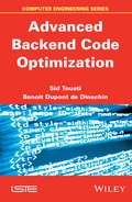
Figure 7.1 illustrates an example. Figure 7.1(a) is the DDG of the straight line code of Figure 7.1(a). If we consider floating point (FP) registers, we highlight values of FP type with bold circles in the DAG. Bold edges correspond to flow dependences of FP type. Once a schedule is fixed as illustrated in Figure 7.1(c), acyclic lifetime intervals are defined as shown in the figure: since we assume a NUAL semantic in this example, lifetime intervals are delayed from the schedule date of the instructions. Remark that the writing clock cycle of a value does not belong to the acylic lifetime interval (which is defined a left open interval), because data cannot be read before finishing the writing.

Figure 7.1. DAG example with acyclic register need

Now, (G) the acyclic register need of type t for the DAG G with respect to (w.r.t.) the schedule σ is the maximal number of values simultaneously alive of type t. (G) is also called MAXLIVE. Figure 7.1(c) shows that we have at most three values simultaneously alive, which are {a, b, d}. Consequently, (G) = 3. The set of a maximal number of values simultaneously alive is called an excessive set, any value belonging to it is called an excessive value.

Computing (G) for a DAG is an easy problem, it is equal to the size of the stable set (maximal clique) in the indirected interference graph shown in Figure 7.1(d). In general, computing the stable set of a graph is NP-complete. But the special case of interval graphs allows us to compute it in [GUP 79].

Once a schedule is fixed, the problem of register allocation is also easy. The number of required registers (chromatic number of the interference graph) of type t is exactly equal to (G), and can be solved due to the algorithm defined in [GUP 79].

As mentioned previously, the acyclic register need has gained a lot of attention in computer science, with good fundamental research results on register allocation with fixed schedules [BOU 06, BOU 07b, BOU 07a]. However, the cyclic problem suffers from a lack of attention from the computer science perspective. The next section defines the cyclic register need and explains our contribution to its formal characterization.

7.3. The periodic register need

When we consider an innermost loop, the DDG G = (V, E) may be cyclic. Each edge e ∈ E becomes labeled by a pair of values (δ(e), λ(e)). δ : E → defines the latency of edges and λ : E → defines the distance in terms of number of iterations. To exploit the parallelism between the instructions belonging to different loop iterations, we rely on periodic scheduling instead of acyclic scheduling. The following section recalls the notations and the notions of SWP.

7.3.1. Software pipelining, periodic scheduling and cyclic scheduling

An SWP is defined by a periodic schedule function σ: V → and an II. The operation u of the ith loop iteration is denoted by u(i), it is scheduled at time σ(u) + i × II. Here, the schedule time σ(u) represents the execution date of u(0) (the first iteration).

The schedule function σ is valid iff it satisfies the periodic precedence constraints

Throughout this part of the book, devoted to register optimization, we also use the terms cyclic or periodic scheduling instead of SWP. If G is cyclic, a necessary condition for a valid SWP schedule to exist is that

where MII is the minimum initiation interval defined by data dependences. Any graph circuit C such that = MII is called a critical circuit.

If G is acyclic, we define MII =1 and not MII = 0. This is because code generation is impossible if MII = 0, because MII = 0 means infinite ILP.

Wang et al. [WAN 94a] modeled the kernel (steady state) of a software pipelined schedule as a two-dimensional matrix by defining a column number cn and a row number rn for each statement. This brings a new definition for SWP, which becomes a triple (rn, cn, II). The row number rn of a statement u is its issue date inside the kernel. The column number cn of a statement u inside the kernel, sometimes called kernel cycle, is its stage number. The last parameter II is the kernel length (initiation interval). This triple formally defines the SWP schedule σ as:

where cn(u) = and rn(u) = σ(u) mod II. In the rest of the chapter, we will write σ = (rn, cn, II) to reflect the equivalence (equality) between the SWP scheduling function σ, defined from the set of statements to clock cycles, and the SWP scheduling function defined by the triple (rn, cn, II).

Let ∑(G) be the set of all valid software pipelined ∑(G) schedules of a loop G. We denote by ∑_L (G) the set of all valid software pipelined schedules whose durations (total schedule time of one original iteration) do not exceed L:

∑(G) is an infinite set of schedules, while ∑_L(G) ⊂ ∑(G) is finite. Bounding the duration L in SWP scheduling allows us, for instance, to look for periodic schedules with finite prologue/epilogue codes, since the size of the prologue/epilogue codes is L – II and 0 ≤ II ≤ L.

7.3.2. The circular lifetime intervals

The value u^t(i) of the ith loop iteration is written u(i) at the absolute time σ(u) + δ_w,t(u) + i × II (starting from the execution date of the whole loop) and killed at the absolute time d_σ (u^t) + i × II. Thus, the endpoints of the lifetime intervals of the distinct operations of any statement u are all separated by a constant time equal to II. Given a fixed period II, we can model the periodic lifetime intervals during the steady state by considering the lifetime interval of only one instance u(i) per statement (say u(0)) that we will simply abbreviate as u.

We recall that the acyclic lifetime interval of the value u ∈ V^R,t is equal to LT_σ(u^t) =]σ(u) + δ_w,t(u), d_σ(u^t)]. The lifetime of a value u ∈ V^R,t is the total number of clock cycles during which this value is alive according to the schedule σ. It is the difference between the death and the birth date, and is given as:

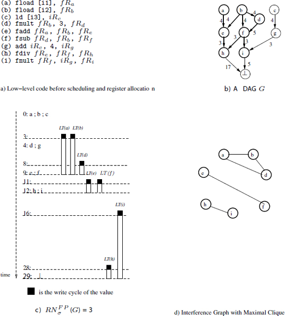
For instance, the lifetimes of v1, v2 and v3 in Figure 7.2 are (respectively) 2, 3 and 6 clock cycles.

Figure 7.2. Periodic register need in software pipelining

The periodic register need (MAXLIVE) is the maximal number of values that are simultaneously alive in the SWP kernel. In the case of a periodic schedule, some values may be alive during several consecutive kernel iterations and different instances of the same variable may interfere. Figure 7.2 illustrates an example: the value v₃ for instance interferes with itself.

Previous results [HEN 92, WER 99] show that the lifetime intervals during the steady state describe a circular lifetime interval graph around the kernel: we wrap (roll up) the acyclic lifetime intervals of the values around a circle of circumference II, and therefore the lifetime intervals become cyclic. We give here a formal definition of such circular intervals.

DEFINITION 7.1.– Circular lifetime interval.– A circular lifetime interval produced by wrapping a circle of circumference II by an acyclic interval I =]a, b] is defined by a triplet of integers (l, r, p), such that:

– l = a mod II is called the left end of the cyclic interval;

– r = b mod II is called the right end of the cyclic interval;

– P = is the number of complete periods (turns) around the circle.

Let us consider the examples of the circular lifetime intervals of v₁, v₂ and v₃ in Figure 7.2(b). These intervals are drawn in a circular way inside the SWP kernel. Their corresponding acyclic intervals are drawn in Figure 7.2(a). The left ends of the cyclic intervals are simply the dates when the lifetime intervals begin inside the SWP kernel. So, the left ends of the intervals of v₁, v₂ and v₃ are 1, 2, 2, respectively (according to definition 7.1). The right ends of the cyclic intervals are simply the dates when the intervals finish inside the SWP kernel. So the corresponding right ends of v₁, v₂ and v₃ are 3, 1, 0, respectively. Concerning the number of periods of a circular lifetime interval, it is the number of complete kernels (II fractions) spanned by the considered interval. For instance, the intervals v₁ and v₂ do not cross any complete SWP kernel; their number of complete periods is then equal to zero. The interval v₃ crosses one complete SWP kernel, so its number of complete period is equal to one. Finally, the definition of a circular lifetime interval is that it groups its left end, right end and number of complete periods inside a triple. The circular interval of v₁, v₂ and v₃ are then denoted as (1, 3, 0), (2, 1, 0) and (2, 0, 1), respectively.

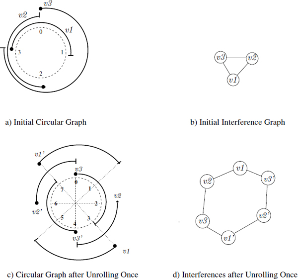
The set of all the circular lifetime intervals around the kernel defines a circular interval graph which we denote by CG(G). As an abuse of language, we use the short term “circular interval” to indicate a circular lifetime interval and the term “circular graph” for indicating a circular lifetime intervals graph. Figure 7.3(a) gives an example of a circular graph. The maximal number of simultaneously alive values is the width of this circular graph, i.e. the maximal number of circular intervals that interfere at a certain point of the circle. For instance, the width of the circular graph of Figure 7.3(a) is 4. Figure 7.2(b) is another representation of the circular graph. We denote by (G) the periodic register need of type t ∈ for the DDG G according to the schedule σ, which is equal to the width of the circular graph.

Figure 7.3. Circular lifetime intervals

7.4. Computing the periodic register need

Computing the width of a circular graph (i.e. the periodic register need) is straightforward. We can compute the number of values simultaneously alive at each clock cycle in the SWP kernel. This method is commonly used in the literature [HUF 93b, JAN 01, NIN 93b, SAW 97, WAN 94b]. Unfortunately, it leads to a method whose complexity depends on the initiation interval II. This factor is pseudo-polynomial, because it does not strictly depend on the size of the input DDG, but rather depends on the specified latencies in the DDG, and on its structure (critical circuit). It is better to use a polynomial method for computing the width of a circular graph, as can be deduced from [HUA 01].

Here, we want to show a novel method for computing the periodic register need whose complexity depends polynomially on the size of the DDG, i.e. it depends only on ||V||, the number of loop statements (number of DDG vertices). This new method will help us to prove other properties (which we will describe later). For this purpose, we find a relationship between the width of a circular interval graph and the size of a maximal clique in the interference graph ¹.

In general, the width of a circular interval graph is not equal to the size of a maximal clique in the interference graph [TUC 75]. This is contrary to the case of acyclic intervals graphs where the size of a maximal clique in the interference graph is equal to the width of the intervals graph. In order to effectively compute this width (which is equal to the register need), we decompose the circular graph (G) into two parts:

1) The first part is the integral part. It corresponds to the number of complete turns around the circle, i.e. the total number of value instances simultaneously alive during the whole steady state of the SWP schedule: ∑_{(l,r,p) a circular interval} p.

2) The second part is the fractional (residual) part. It is composed of the remainder of the lifetime intervals after removing all the complete turns (see Figures 7.3(b) and (c)). The size of each remaining interval is strictly less than II, the duration of the SWP kernel. Note that if the left end of a circular interval is equal to its right end (l = r), then the remaining interval after ignoring the complete turns around the circle is empty (]l, r] =]l, l] = ). These empty intervals are then ignored from this second part. Two classes of intervals that remain are as follows:

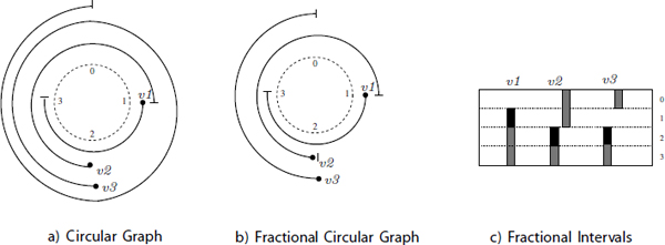
These two classes of intervals define a new circular graph. We call it a fractional circular graph because the size of its lifetime intervals is less than II. This circular graph contains the circular intervals of the first class, and those of the second class after merging the left part of each interval with its right part (see Figure 7.3(b)).

DEFINITION 7.2.– Fractional circular graph.– Let (G) be a circular graph of a DDG G = (V, E). The fractional circular graph, denoted by (G), is the circular graph after ignoring the complete turns around the circle:

We call the circular interval (l, r) a circular fractional interval. The length of each fractional interval (l, r) ∈ (G) is less than II clock cycles. Therefore, the periodic register need of type t is equal to:

[7.1]

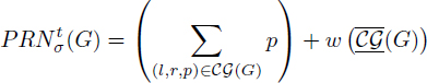
where w denotes the width of the fractional circular graph (the maximal number of values simultaneously alive). Computing the first term of formula [7.1] (complete turns around the circle) is easy and can be computed in linear time (provided lifetime intervals) by iterating over the ||V^R,i|| lifetime intervals and adding the integral part of .

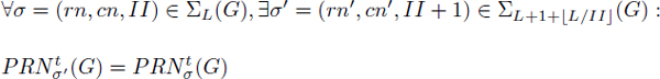
However, the second term of formula [7.1] is more difficult to compute in polynomial time. This is because, as stated before, the size of a maximal clique (in the case of an arbitrary circular graph) in the interference graph is not equal to the width of the circular interval graph [TUC75]. In order to find an effective algorithmic solution, we use the fact that the fractional circular graph (G) has circular intervals that do not make complete turns around the circle. Then, if we unroll the kernel exactly once to consider the values produced during two successive kernel iterations, some circular interference patterns become visible inside the unrolled kernel. For instance, the circular graph of Figure 7.4(a) has a width equal to 2. Its interference graph in Figure 7.4(b) has a maximal clique of size 3. Since the size of these intervals does not exceed the period II, we unroll the circular graph once as shown in Figure 7.4(c). The interference graph of the circular intervals in Figure 7.4(d) has a size of a maximal clique equal to the width, which is 2: note that v2 does not interfere with because, as said before, we assume that all lifetime intervals are left open.

When unrolling the kernel once, each fractional interval (l, r) ∈ (G) becomes associated with two acyclic intervals I and constructed by merging the left and the right parts of the fractional interval of two successive kernels. I and are then defined as follows:

– If r ≥ l, then I =]l, r] and =]l + II, r + II].

– If r < l, then I =]l, r + II] and =]l + II, r + 2 × II].

THEOREM 7.1.– [TOU 07, TOU 02] Let (G) be a circular fractional graph (no complete turns around the circle exists). For each circular fractional interval (l, r) ∈ (G), we associate the two corresponding acyclic intervals I and . The cardinality of any maximal clique in the interference graph of all these acyclic intervals is equal to the width of (G).

The next section presents some of the mathematical results that we proved due to equation [7.1] and theorem 7.1.

Figure 7.4. Relationship between the maximal clique and the width of a circular graph

7.5. Some theoretical results on the periodic register need

In this section, we show how to compute the minimal periodic register need of type t for any valid SWP independently of II. We call it the periodic register sufficiency. We define it as:

[7.2]

where ∑(G) is the set of all valid SWP schedules for G.

Computing the periodic register sufficiency allows us, for instance, to determine if spill code cannot be avoided for a given loop: if is the number of available registers of type t, and if PRF^t(G) > then there are not enough registers to allocate to any loop schedule. Spill code has to be introduced necessarily, independently of II.

Let us start by characterizing a relationship between minimal periodic register need for a fixed II.

7.5.1. Minimal periodic register need versus initiation interval

The literature contains many SWP techniques about reducing the periodic register need for a fixed II. It is intuitive that, the lower the initiation interval II, the higher the register pressure, since more parallelism requires more memory. If we succeed in finding a software pipelined schedule σ which needs R^t = (G) registers of type t, and without assuming any resource conflicts, then it is possible to get another software pipelined schedule that needs no more than R^t registers with a higher II. We prove here that increasing the maximal duration L is a sufficient condition, bringing the first formal relationship that links the periodic register need, the II and the duration. Note that the following theorem has been proved when δ_w,t = δ_r,t = 0 only (no delay to access registers).

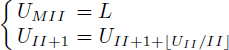
THEOREM 7.2.– [TOU 07, TOU 02] Let G = (V, E) be a loop DDG with zero delays in accessing registers (δ_r,t = δ_w,t = 0). If there exists an SWP σ = (rn, cn, II) that needs R^t registers of type t having a duration at most L, then there exists an SWP σ′ = (rn′, cn′, II + 1) that needs R^t registers also having at most a duration L′ = L + 1 + . Formally:

7.5.2. Computing the periodic register sufficiency

The periodic register sufficiency defined by equation [7.2] is the absolute register sufficiency because it is defined for all valid SWP schedules belonging to ∑(G) (an infinite set). In this section, we show how to compute it for a finite subset ∑_L(G) ∑(G), i.e. for the set of SWP schedules such that the duration does not exceed L. This is because many practical SWP schedulers assume a bounded duration L in order to limit the code size. However, we can choose a sufficiently large value for L such that:

Some existing solutions show how to determine the minimal register need given a fixed II [ALT 95, FIM 01, SAW 97, TOU 04]. If we use such methods to compute periodic register sufficiency, we have to solve many combinatorial problems, one for each II, starting from MII to a maximal duration L. Fortunately, the following corollary states that it is sufficient to compute the periodic register sufficiency by solving a unique optimization problem with II = L if we increase the maximal duration (the new-maximal duration is denoted L′ to distinguish it from L). Let us start by the following lemma, which is a direct consequence of theorem 7.2:

LEMMA 7.1.– [TOU 07, TOU 02] Let G = (V, E) be a DDG with zero delays in accessing registers. The minimal register need (of type t ∈ ) of all the software pipelined schedules with an initiation interval II assuming duration at most L is greater than or equal to the minimal register need of all the software pipelined schedules with an initiation interval II′ = II + 1 assuming duration at most L′ = L + 1 + . Formally,

COROLLARY 7.1.– [TOU 07, TOU 02] Let G = (V, E) be a DDG with zero delays in accessing registers. Then, the exact periodic register sufficiency of G (of type t) assuming duration at most L is greater than or equal to the minimal register need with II = L assuming duration at most L′ ≥ L. L′ is computed formally as follows:

where L′ is the (L – MII)^th term of the following recurrent sequence (L′ = U_L):

In other words, corollary 7.1 proves the following implication:

where the value of L′ is given by corollary 7.1.

7.5.3. Stage scheduling under register constraints

Stage scheduling, as studied in [EIC 96], is an approach that schedules loop operations given a fixed II and a fixed reservation table (i.e. after satisfying resource constraints). In other terms, the problem is to compute the minimal register need given a fixed II and fixed row numbers (rn), while column numbers (cn) are left free (i.e. variables to optimize). This problem has been proved NP-complete by Huard [HUA 01]. A careful study of his proof allows us to deduce that the complexity of this problem comes from the fact that the last readers (consumers) of the values are not known before scheduling the loop. Huard in [HUA 01] has already claimed that if the killer is fixed, then stage scheduling under register constrains is a polynomial problem. Mangione-Smith [MAN 92] proved that stage scheduling under register constraints has a polynomial time complexity in the case of data dependence trees and forest of trees. This section proves a more general case than [MAN 92] by showing that if every value has a unique killer (last consumer) known or fixed before instruction scheduling, as in the case of expression trees, then stage scheduling under register constraints is a polynomial problem. This claim was already known by few experts; here we provide a straightforward proof using the formula of periodic register need given in equation [7.1].

Before proving this general case, we first start by proving it for the case of trees (for clarity).

Let us begin by writing the formal problem of SWP with register need minimization. Note that the register type t ∈ is fixed, performing a stage scheduling among all register types conjointly remains an open problem.

[7.3]

This standard problem has been proved NP-complete in [EIS 95a], even for trees and chains. Eichenberger et al. studied a modified problem by considering a fixed reservation table. By considering the row and column numbers (σ(u) = rn(u) + II × cn(u)), fixing the reservation table amounts to fixing row numbers while letting column numbers as free integral variables. Thus, by considering the given row numbers as conditions, problem [7.3] becomes:

[7.4]

That is,

[7.5]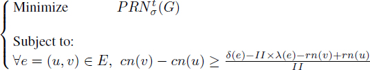

It is clear that the constraints matrix of problem [7.5] constitutes an incidence matrix of the graph G. If we succeed in proving that the objective function (G) is a linear function of the cn variables, then problem [7.5] becomes an integer linear programming system with a totally unimodular constraints matrix, and consequently, it can be solved with polynomial time algorithms [SCH 87]. Since the problem of stage scheduling defined by problem [7.5] has been proved NP-complete, it is evident that (G) cannot be expressed as a linear function of cn for an arbitrary DDG. In this section, we restrict ourselves to the case of DDGs where each value u ∈ V^R,t has a unique possible killer , such as the case of expression trees. In an expression tree, each value u ∈ V^R,t has a unique killer that belongs to the same original iteration, i.e. λ ((u, )) = 0. With this latter assumption, we will prove in the remaining of this section that (G) is a linear function of column numbers.

Let us begin by recalling the formula of (G)

[7.6]

The first term of the equation corresponds to the total number of turns around the circle, while the second term corresponds to the maximal fractional intervals simultaneously alive (the width of the circular fractional graph). We set P = ∑(l, r, p)∈(G) p and W = w ((G)).

We know that ∀(l, r, p) ∈ (G) the circular interval of a value u ∈ V^R,t, its number of turns around the circle is p = = .

Since each value u is assumed to have a unique possible killer belonging to the same original iteration (case of expression trees),

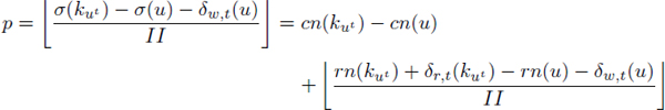
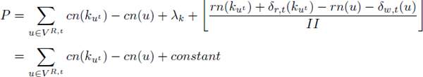
Here, we succeed in writing P = ∑p as a linear function of column numbers cn, since rn and II are constants in problem [7.5]. Now, let us explore W. The fractional graph contains the fractional intervals {(l, r)|(l, r, p) ∈ (G)}. Each fractional interval (l, r) of a value u ∈ V^R,t depends only on the row numbers and II as follows:

As can be seen, the fractional intervals depend only on row numbers and II, which are constants in problem [7.5]. Hence, W, the width of the circular fractional graph is a constant too. From all the previous formulas, we deduce that:

yielding to:

[7.7]

Equation [7.7] rewrites problem [7.5] as the following integer linear programming system (by neglecting the constants in the objective function):

[7.8]

The constraints matrix of system [7.8] describes an incidence matrix; so it is totally unimodular. It can be solved with a polynomial time algorithm.

This section proves that stage scheduling of expression trees is a polynomial problem. Now, we can consider the larger case of the DDGs assigning a unique possible killer for each value u^t of type t. Such a killer can belong to a different iteration λ_k = λ((u, )). Then, the problem of stage scheduling in this class of loops remains also polynomial as follows:

Since II and row numbers are constants, W remains a constant as proved by the following formulas of fractional intervals:

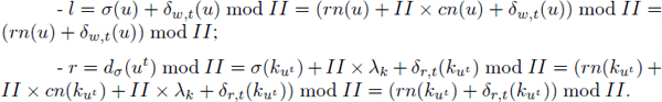
Consequently, (G) remains a linear function of column numbers, which means that system [7.8] can still be solved via polynomial time algorithms (usually with network flow algorithms).

Figure 7.5. Examples of DDG with unique possible killer per value

Our result in this section is more general than expression trees. We extend the previous result [MAN 92] in two ways. Figure 7.5 shows some examples, where all edges are flow dependences labeled by the pairs (δ(e),λ(e)).

The Register Need of a Fixed Instruction Schedule 139

1) Cyclic DDGs: our result takes into account cyclic DDGs with a unique killer per value. As an example, Figure 7.5(a) is a cyclic DDG with a unique possible killer per value. Such DDG is not considered in [MAN 92], because it is cyclic while it is neither a tree nor an acyclic DDG.

2) Acyclic DDG: our result also takes into account acyclic DDGs with a unique possible killer per value, which are not necessarily trees or forest of trees. For instance, Figure 7.5(b) and Figure 7.5(c) are examples of acyclic DDG where every node has a unique possible killer (because of the transitive relationship between nodes). These DDGs are not trees. Analyzing such unique killer relationships in general acyclic DDGs can be done using the so-called potential killing relation, which has been formally defined in [TOU 05, TOU 02]. In Figure 7.5(b), we have the following unique killers: = d, = e. In Figure 7.5(c), we have the following unique killers: = e, = e.

7.6. Conclusion on the register requirement

The register requirement of a DAG in acyclic scheduling is a well-studied topic: when the schedule is fixed, the register requirement (MAXLIVE) is exactly equal to the number needed for register allocation. So nothing new is introduced here. The case of fixed schedules for arbitrary codes (with possible branches) is a distinct problem, since the notion of MAXLIVE is not precise statically when the compiler cannot guess the taken branch. Consequently, computing the minimal number of allocated registers needs sophisticated algorithms as proposed in [BOU 06, BOU 07b, BOU 07a].

The periodic register requirement in cyclic scheduling has got less fundamental results in the literature, compared to the acyclic case. The work presented in this chapter analyzes some of our results published in [TOU 07]. The first contribution brings a polynomial method for computing the exact register need ( (G)) of an already scheduled loop. Given a register type t ∈ , the complexity to compute (G) is , where V^R,t is the number of loop statements writing a value of type t. The complexity of the cited methods depends on II, which is a pseudo-polynomial factor. Our new formula to compute (G) in polynomial time does not really solve an open problem; it, however, allows us to deduce other formal results explained below.

A second contribution provides a sufficient condition so that the minimal register need under a fixed II does not increase when incrementing II. We gave in [TOU 07] an example to show that it is sometimes possible that the minimal register need increases when II is incremented. Such situations may occur when the maximal duration L is not relaxed (increased). This fact contradicts the general thought that incrementing II would require fewer registers (unless the constraint on L is loosened).

Guaranteeing that the register need is a non-increasing function versus II when relaxing the maximal duration allows us now to easily write the formal problem of scheduling under register constraints instead of scheduling with register minimization as usually done in the literature. Indeed, according to our results, we can finally apply a binary search on II. If we have , a fixed number of available registers of type t, and since we know how to increase L so as the curve of (G) versus II becomes non-increasing, we can use successive binary search on II until reaching a (G) below . The number of such binary search steps is at most lg₂ (L).

A third contribution proves that computing the minimal register need with a fixed II = L is exactly equal to the periodic register sufficiency if L sufficiently large, i.e. the minimal register need of all valid SWP schedules. Computing the periodic register sufficiency (PRF^t (G)) allows us to check for instance if introducing spill code is unavoidable when PRF^t (G) is greater than the number of available registers.

While stage scheduling under registers constraints for arbitrary loops is an NP-complete problem, the fourth and final contribution gives a straightforward proof that stage scheduling with register minimization is a polynomial problem in the special case of expression trees, and generally in the case of DDGs providing a unique possible killer per value. This general result has already been claimed by few experts, but a simple proof of it is made possible due to our polynomial method of (G) computation.

This chapter proposes new open problems. First, an interesting open question would be to provide a necessary condition so that the periodic register need would be a non-increasing function of II. Second, in the presence of architectures with non-zero delays in accessing registers, is theorem 7.2 still valid? In other words, can we provide any guarantee that minimal register need in such architectures does not increase when incrementing II? Third, we have shown that there exists a finite value of L such that the periodic register sufficiency assuming a maximal duration L is equal to the absolute periodic register sufficiency without assuming any bound on the duration. The open question is how to compute such appropriate value of maximal duration. Fourth and last, we require a DDG analysis algorithm to check whether each value has one and only one possible killer. We have already published such an algorithm for the case of DAG in [TOU 05], but the problem here is to extend it to loop DDG.

The next chapter (Chapter 8) studies the notion of register saturation, which is the maximal register requirement of a DDG, for all possible valid schedules.

1 Remember that the interference graph is an undirected graph that models interference relations between lifetime intervals: two statements u and v are connected iff their (circular) lifetime intervals share a unit of time.