
CHAPTER 15
A Simple Frequency Counter
In this chapter we construct a simple device for measuring frequency called a frequency counter. It uses the timer function in the Arduino’s Atmel processor and measures frequencies from the audio range to a little over 6 MHz. It is constructed on a single Arduino R3 prototyping shield and includes an LCD to readout the frequency. The counter is surprisingly accurate and can easily be calibrated with a known accurate frequency source. The chapter ends with a discussion of how to use the frequency counter with a typical QRP radio that lacks a frequency readout. We use the Arduino Frequency Counter to measure the Variable Frequency Oscillator or “VFO” frequency and then display the corresponding receive or transmit frequency on an LCD. The frequency counter is a nice addition to many low-cost QRP rigs. Figure 15-1 shows the frequency counter being used with an MFJ 40 Meter Cub QRP transceiver. In this case we use the Arduino to do a little bit of math to convert the VFO frequency to the actual frequency of the radio. We will discuss this in greater detail later in this chapter.
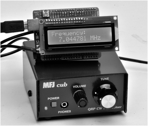
FIGURE 15-1 The Arduino frequency counter connected to an MFJ Cub QRP transceiver.
There are some indispensable tools that we use when working with radio gear. There are the obvious ones: side cutters, pliers, screwdrivers, soldering iron, and so on. A good multimeter is a useful tool as well. One tool that doesn’t get much mention but is equally useful to the multimeter is a frequency counter. The name is a bit of a misnomer because you don’t really count frequencies. What you are doing instead is counting the number of transitions, or “cycles,” a signal makes over a known period of time. From the count we determine the frequency.
Frequency is nothing more than expressing the “cycles per second” or “Hertz” of a signal. So, if we measure 3000 transitions of a waveform over a period of one second, the result is 3000 cycles per second. Or is it? Take a look at Figure 15-2 depicting a sine wave. We see that there are actually TWO transitions in each “cycle,” one “rising” and one “falling.” So, what do we actually measure? We don’t measure ALL of the transitions. Instead we count the cycles using only the rising or falling edge of the signal. If we count only the rising edges of the 3000 cycles per second signal, we actually count 3000 transitions.
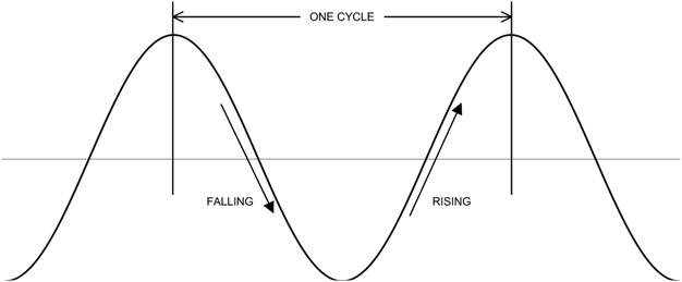
FIGURE 15-2 Transitions in a sine wave.
But wait, there’s more! Counting and timing are two things that a processor can do well. Arduino is no exception. It turns out that the Atmel processors used in the Arduino have a clever little added bonus; the controllers have internal programming that allows the hardware to count transitions on an input without the need for external software via a dedicated hardware function! All we have to do is turn it on and turn it off to perform the count and then read back the results.
Of course, the Atmel processor is a digital device and the counter hardware function is implemented on a digital IO pin. To be more specific, digital pin 5 implements the hardware counting function. However, the sine wave depicted in Figure 15-2 is an analog signal and may have varying amplitude; therefore, we must do something to convert the analog signal into something more compatible with the digital input. One way to convert the sine wave to a digital signal is with a comparator (a device that when the input exceeds a set threshold, the output, normally zero or low, goes high). Another method is to use a high gain amplifier and have the input signal drive the amplifier into “saturation,” meaning that as soon as the input rises above zero, the output goes full “on” or is saturated. It is the saturation method we have chosen to “condition” our input signal so that the Arduino may count the transitions. Figure 15-3 shows how the sine wave is “transformed” into a digital square wave for the counter.
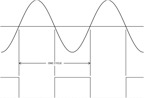
FIGURE 15-3 Deriving a digital signal from the sine wave.
Circuit Description
The input conditioning circuit for the frequency counter is shown in Figure 15-4. Two BC547B NPN bipolar transistors, Q1 and Q2, are cascaded to provide sufficient gain that a relatively low level signal produces adequate signal level to pin 5 of the Arduino for the counter to function. Table 15-1 is the parts list for the frequency counter.
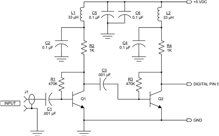
FIGURE 15-4 Frequency counter shield schematic.
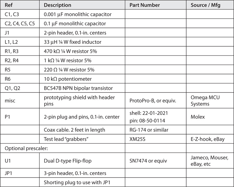
TABLE 15-1 Parts List for the Frequency Counter
Constructing the Shield
You may have noticed from the schematic (Figure 15-4) that the frequency counter uses digital input pin 5 and that we have already used this pin for the LCD display in Chapter 3. True, but pins in conflict is something that we encounter time and time again while working with Arduino and Arduino-related projects. What can we do? As designers, we do the best job we can of optimizing re-use of the preceding projects in constructing new projects, but we can’t always win. You may recall that we discussed the issues with “deconflicting” pins in Chapter 10, “Project Integration.” But, for this project, we have decided to use a dedicated LCD on the frequency counter shield, thus mitigating the conflict between pins.
The component layout for the frequency counter shield is shown in Figure 15-5. We have constructed the frequency counter shield on a ProtoPro-B prototyping shield. In laying out the components for the shield, we encounter several issues. First, we must allow space for the large amount of real estate taken up by the LCD on the shield. Having the LCD mounted on the shield means that we need to use some low-profile construction techniques. You could, of course, make the LCD removable. The second issue is with regards to good high-frequency design. We bring high-frequency signals into the frequency counter shield and it is important that we keep these signals from affecting other parts of the Arduino. Good construction practice is that we keep leads short and that we bypass all power leads. These practices do not completely eliminate RF signals from getting into places we don’t want them; however, they reduce the chances of our getting into trouble with stray RF. Of course, you can also take this project and mount it in a nice shielded enclosure.
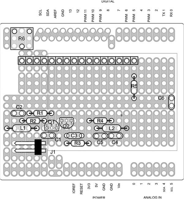
FIGURE 15-5 Frequency counter shield component layout.
The input cable for the counter is made from a piece of coax such as RG-174 or similar flexible, lightweight coax, that is terminated on a 2-pin Molex socket that connects to J1. Our test cable is about 2 ft in length. The Molex shell is a part number 22-01-2021 and the pins are part number 08-50-0114. The pins are a crimp-style part; however, if you don’t have the correct crimping tool, you can solder them or crimp them carefully using a pair of needle nose pliers. The shell and pins are available from Mouser Electronics (www.mouser.com) and other places such as eBay. They are inexpensive and we use similar Molex parts in other projects in this book. This series of Molex connectors mates nicely with the 0.10-in. header pins that we use. You can terminate the other end of the coax with alligator clips.
Looking at Figure 15-6, the wiring diagram for the frequency counter shield, we see that pin 5 has been reused as the input for the frequency counter and that LCD data pins, DB4 through DB7, have been relocated to digital pin 6 through 9. As you might expect, the software (Listing 15-1) must also reflect this change in defining the data pins assigned to the LCD. We found that creating an Excel worksheet really helps in solving pin conflicts, but sometimes, there are no solutions. You can see our worksheet in Appendix C. While many pins on the Arduino serve multiple functions, some, like the hardware counting functions, are only available on dedicated pins, in this case, digital pin 5. The completed shield is shown in Figure 15-7.
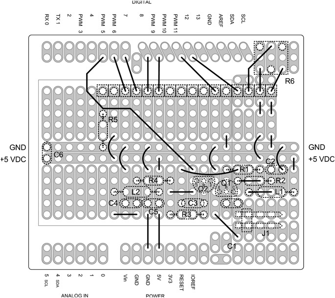
FIGURE 15-6 Frequency counter shield wiring.
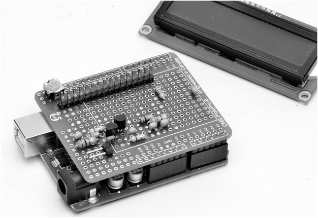
FIGURE 15-7 The completed frequency counter shield.
An Alternate Design for Higher Frequencies
One of the limitations of the Arduino and in particular the Atmel ATmega328 processor family is the maximum rate at which the timer can count. Using a 16 MHz clock rate (normal for the Arduino Duemilanove and Uno), the maximum frequency that can be expected to be read is a little above 6 MHz. So, if we want to measure higher frequencies, what do we do?
One alternative is to add a prescaler to the counter. The prescaler goes between the input signal conditioning transistor and digital pin 5. We use a binary counter to divide the frequency down to a range that can be measured. In this case, we are adding a TTL Dual D-Type Flip-Flop, an SN7474 14 Pin DIP part. A single D-Type Flip-Flop is configured as a “divide by two” counter by connecting the Q “NOT,” or Q “bar” output, to the “D” input of the Flip-Flop and applying the input pulses to the clock input. The “Q” output is half the rate of the input pulse rate. Figure 15-8 shows both halves of an SN7474 Dual Flip-Flop configured as a divide by four counter and inserted between the collector of Q1, the input transistor, and digital pin 5 of the Arduino. Thus, for every four pulses of the input waveform, the Arduino counts only one. So, instead of being limited to a little over 6 MHz on our counter, we can now measure frequencies to approximately 24 MHz. Jumper JP1 in Figure 15-8 is used to select between divide by two or divide by four. A CMOS Dual D-Type Flip-Flop, the CD4013B, can be used as an alternative to the TTL SN7474. Either part works; however, the CD4013B has a different pinout than the SN7474.

FIGURE 15-8 Divide by four prescaler using two D-Type Flip-Flops.
Figures 15-9 and 15-10 show the way we built the “prescaler” with a parts layout and wiring for this add-on design. To read the correct frequency on the LCD, we also made a modification to the software to multiply the count by one, two, or four by uncommenting the appropriate #define statement. This means that the prescaler is selectable when you compile the software.
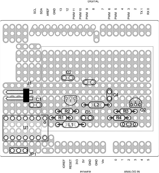
FIGURE 15-9 Parts layout for the prescaled frequency counter.
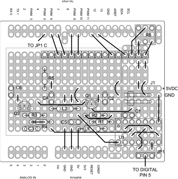
FIGURE 15-10 Wiring diagram for the prescaled frequency counter.
Code Walk-Through for Frequency Counter
By this time, you have seen many different Arduino programs, and they all follow much the same basic structure. The frequency counter is no different. We start out with some definitions and then follow that with the initialization of the LCD in setup() and then the main body of the program is loop(). The only new item in this program is a new library, FreqCounter.h. Download the library using this link:
http://interface.khm.de/wp-content/uploads/2009/01/FreqCounter_1_12.zip
and unzip the file into your library directory in the same manner as with other new libraries (e.g., Chapter 4).
The source code for the frequency counter is provided in Listing 15-1. The design is based on work done by Martin Nawrath from the Academy of Media Arts and utilizes the FreqCounter.h library created by Martin. The library uses the ATmega328 programmable timers, TIMER/COUNTER1 to count the transitions on digital pin 5, and TIMER2 to set the gate time.
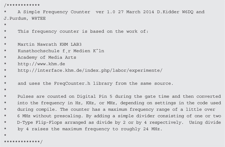
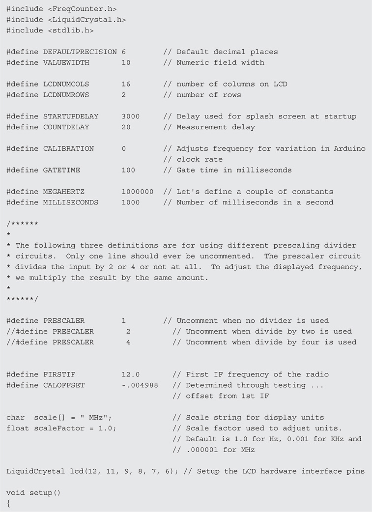
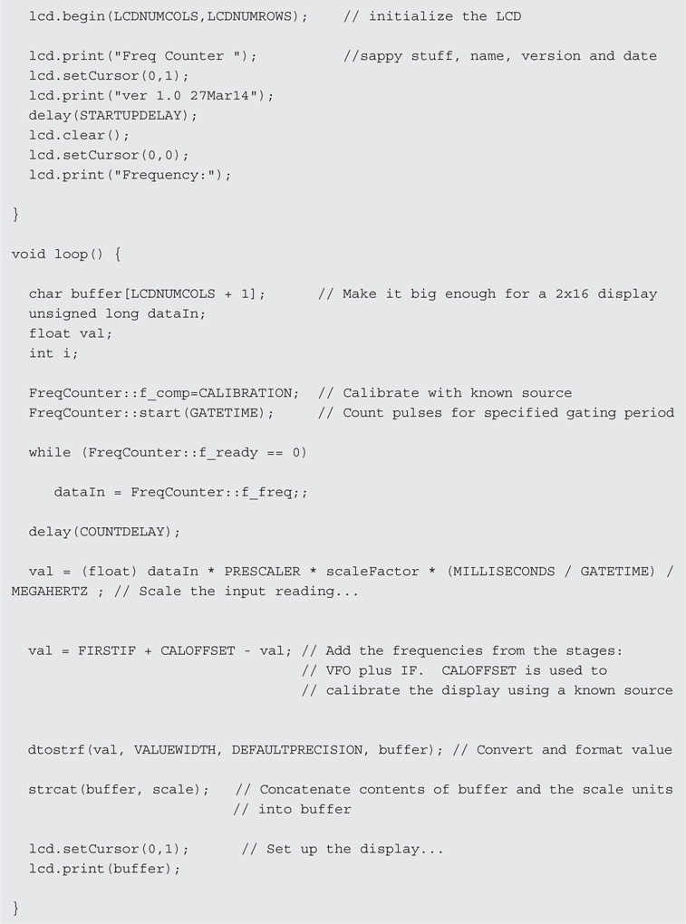
LISTING 15-1 Frequency counter source listing.
Essentially, TIMER2 is set up to count clock ticks to equal the preset gate time. During the period of time that TIMER2 is counting, TIMER/COUNTER1 is counting the rising edge transitions on digital pin 5. Once the count is completed, the value is passed back to the program.
The returned value is converted to an actual frequency (cycles per second, or Hertz) by multiplying the number of gate times in one second, in this case 1000 milliseconds divided by 100 milliseconds gate time or 10, and then the result is divided by 10E6 to obtain the result in megahertz (MHz). The resulting frequency is then cast as a floating point number.
We use the stdlib.h functon, dtostrf() to convert from the float value to an ASCII text string and stuff the result into buffer. We then concatenate the contents of buffer with the scale units string (MHz) and then output the contents of buffer to the display.
One thing to note: The resolution of the counter is determined by the gate time. With a gate time of 100 milliseconds, the counter is limited to 10 Hz resolution. To increase the resolution to 1 Hz, the gate time is changed to 1 second by setting the value of GATETIME to 1000.
Displaying the Tuned Frequency of Your Display-less QRP Rig
There are a number of QRP radios that take a minimalist approach in their design and as a result have no frequency display. For many of these rigs, it is a fairly simple matter to connect a frequency counter, such as the one described in this project, to obtain a direct frequency readout. We describe how to connect the Arduino Frequency Counter to a typical QRP radio and then give several examples.
There are several different approaches to the design of QRP radios. The simplest is the “direct conversion” or “zero IF” receiver/transmitter, but more and more dual-conversion transceivers are being built because availability of low-cost circuits like the SA602/SA612 Double Balanced Mixer/Oscillator chip. We discuss the dual-conversion applications first and then the direct conversion sets. We show how the Arduino Frequency Counter is connected to several popular QRP radios available today. We have selected the MFJ Cub QRP Transceiver as an example. The Cub has six different models, each a single band transceiver.
Double Conversion Applications
The majority of QRP radios these days use a double conversion scheme. The availability of low-cost mixer/oscillator combination chips, such as the SA602, has made it very economical and provides a high degree of stability and performance. But, many times what comes with the low cost is no frequency display. You get a radio with a tuning knob. And with that, you have no idea where you are on the band. What these radios need is a frequency display.
The double conversion receiving scheme is shown in Figure 15-11. A double conversion transmitter would be very similar, with the signal flow in the opposite direction. The first mixer combines the incoming signal with the VFO to produce a signal in the intermediate frequency or “IF” passband. The second mixer combines the output of the IF with the BFO (Beat Frequency Oscillator) to produce the recovered audio signal. The key elements of this project are determining the frequency of the VFO and the IF. The IF is a fixed frequency and should be known from the radio design. The VFO is variable and is what we want to measure with the frequency counter. In many cases, the transmitter is also controlled by the same VFO as the receiver, but the second mixer may be separate and operating at a slightly different frequency than the receiver. Why is the transmitter on a different frequency? Often we use the transmitted signal as a sidetone to monitor our sending by leaving the receiver operating but with greatly attenuated output. If there was no offset between the transmitted and received frequencies, we would hear a tone of zero Hz. A better way to state this is that the resulting tone would be zero Hz and we can’t hear that.
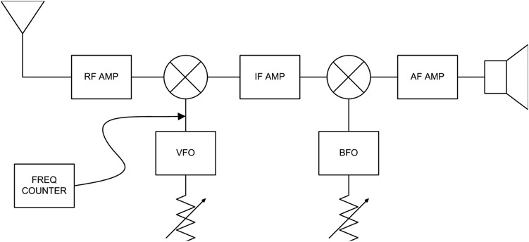
FIGURE 15-11 Double conversion scheme.
It may actually be more important to know the transmitted frequency rather than the received frequency. Many times, this choice really depends on the design of the radio and how accessible the transmit frequency is. In either case, the methodology remains the same.
As an example, let’s use a radio operating at 14 MHz with a 5 MHz IF. Assume the radio tunes 14.000 through 14.070 MHz. With these numbers in mind, the VFO operates at the difference of the two frequencies; therefore when the radio is tuned to 14.000, the VFO is 14.000 minus 5.000, yielding a difference of 9 MHz. We use the frequency counter to measure the VFO frequency (i.e., 9 MHz) and that result is added to the IF (i.e., 5 MHz) and the sum of these two values is the radio’s frequency (14 MHz). Again, there may be small offsets introduced between transmit and receive to provide a sidetone frequency on transmit, but these can be determined and taken into account when the display frequency is calculated. Because the IF is fixed, if we know the result at one VFO setting, we use the same calculation at any VFO setting for this radio on this band.
Adding a Frequency Display to the MFJ Cub QRP Transceiver
MFJ has a series of single-band QRP radios. These offer some good performance for the cost, but they do lack a frequency display. We chose to add the frequency display to the 40 Meter Cub, the MFJ 9340 transceiver. From the information provided by MFJ in the Cub’s manual, the VFO operates in the 5 MHz range and the IF is 12 MHz. Different bands use different combinations of VFO and IF frequencies as illustrated in Table 15-2.
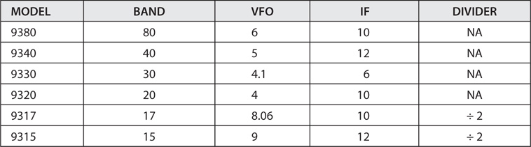
TABLE 15-2 MFJ Cub Transceiver VFO and IF Frequencies
When the VFO frequency is less than 6 MHz, the counter is used without a divider stage; hence the NA entries in Table 15-2. For the Cub, only two models require a divider: 9317 and 9315. A divide by 2 circuit is sufficient in these two cases.
As it turns out, the Cub makes it very easy to add the frequency display. In this case, we monitor the transmit frequency. The Cub uses an SA602 Mixer/Oscillator for the first mixer and VFO as shown in the partial schematic in Figure 15-12. The output of the oscillator not only is used in the receiver’s first mixer, it is passed to the transmitter through a buffer transistor, Q4. The buffer is always on so we can monitor the transmit frequency all the time. Transmit power level is controlled by the divider network of R18 and R19. We tap into the transmit VFO across the pot, R19. Figure 15-13 shows how we installed a small length of RG-174 coax from our tie point on R19 to an RCA jack to access the VFO buffer output. We drilled a new hole and mounted the RCA jack on the rear panel. Figure 15-14 is a close-up, showing the center conductor of the coax (the white lead) connected to the “hot” side of the pot, R19. The coax shield is connected to the ground side of the pot and is the black wire
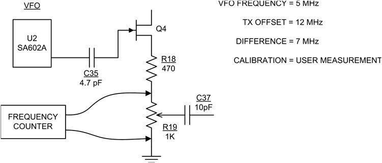
FIGURE 15-12 Attaching the frequency counter to the MFJ Cub transceiver.
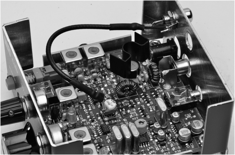
FIGURE 15-13 The “pickoff point” from the frequency counter in the MFJ Cub. (Cub courtesy of MFJ Enterprises)
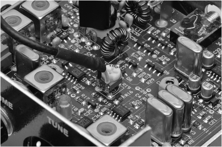
FIGURE 15-14 Close-up of the pickoff installed in the 40 Meter MFJ Cub QRP transceiver.
One thing to note: When the frequency counter is attached to the Cub, the VFO frequency is “pulled” off slightly. This is to be expected, as even with the buffer stage our circuit loads down the oscillator in the SA602. This is not a big deal, but we have to account for it in our calibration adjustments.
Calibration of the frequency counter with the Cub is accomplished using a known reference source. The most readily available known reference is a good communications receiver. With the 40 Meter Cub, we set the receiver to 7.000 MHz. Depending on which model Cub is used, set the receiver to the appropriate frequency. The Cub is connected to a 50 Ohm dummy load (e.g., Chapter 6) and the frequency counter. Tune the Cub to zero beat on the receiver while transmitting a signal. A frequency close to the expected 7.000 MHz frequency should appear on the LCD. Once the signal is zero beat on the receiver, note the displayed frequency on the Arduino LCD. The difference between the displayed frequency and the receiver’s 7.000 is the calibration offset that is used in the frequency counter. It is important to note whether the displayed value is larger or smaller than the receiver’s frequency as this difference determines whether the adjustment, or “offset,” is added to or subtracted from the frequency counter’s displayed value. The offset is used for the CALOFFSET definition in the program.
Adding a Frequency Display to a NorCal 40
The NorCal 40, developed by Wayne Burdick (N6KR) of Elecraft fame, was originally distributed by the Northern California QRP Club. The NorCal 40 is now available through Wilderness Radio (http://www.fix.net/~jparker/wild.html). This is a very popular radio and many of them have been sold over the years. The NorCal 40 does lack a frequency display, and adding one is fairly simple. Figure 15-15 shows the frequency plan of the radio.

FIGURE 15-15 NorCal 40A partial block diagram showing frequency plan.
The NorCal 40A uses a VFO covering the range of 2.085 to 2.125 MHz giving a tuning range of 40 kHz. The VFO is mixed with a 7.000 MHz incoming signal, the difference producing the IF of 4.9150 MHz. The IF is mixed with the BFO at 4.9157 MHz, the difference being 700 Hz, which is a pleasant pitch for copying Morse code on CW. The transmit scheme is the reverse, but with a slightly different mixer frequency. For 7.000 MHz out, the 2.085 MHz VFO is mixed with 4.9150, the sum being 7.000 MHz. By using a separate TX LO and RX BFO that differ by 700 Hz, the receive frequency is offset to provide sidetone and a pleasant tone for reception.
Figure 15-16 is a partial schematic of the NorCal 40A showing the best points to connect the frequency counter. JFET Q8 is the common VFO and the frequency counter is connected across the RF choke (RFC2) connected to Q8’s source lead. Just as we did with the Cub, we use a short length of RG174 coax, connecting the center conductor to the Q8 source side and the shield braid to the ground side of RFC2. The value in the program for PRESCALER is set to 1 and for FIRSTIF is set to 4.9150. Again, the value for CALOFFSET must be determined by testing.
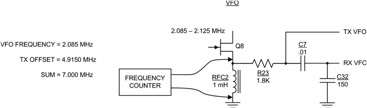
FIGURE 15-16 NorCal 40A partial schematic showing connection for frequency counter.
Direct Conversion Applications
There are a number of Direct Conversion (DC) radio designs available. Figure 15-17 shows how a direct conversion receiver is configured. For the sake of clarity, only the receiver is shown. The receiver consists of an RF amplifier stage followed by a mixer. The VFO is operating at close to the same frequency as the incoming signal. The output is the difference between the frequency of the incoming signal and the VFO frequency. What we want in the output is in the audio range, so if the VFO is close to the received frequency (in other words, within a kHz or so), the difference is an audio signal. We can measure the frequency of the VFO and have a pretty good idea of the received frequency. It won’t be exact because we designed the receiver to be slightly off frequency so that we would recover an audio output. If the VFO were exactly the same as the incoming frequency, the difference would be zero and there would be no recovered signal.
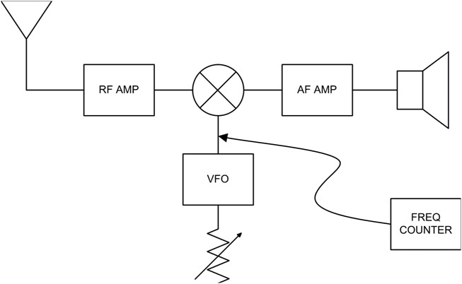
FIGURE 15-17 Direct conversion scheme.
Because a DC radio uses a common VFO for transmit and receive, the transmitted frequency is the same as the receive frequency. Generally this causes a problem in that when the received and transmitted signals are on the same frequency, there is no difference signal to be heard as audio. The recovered signal is zero Hz. Many DC radios use a TX offset to move the transmitted frequency slightly away from the received frequency in order to have enough difference to produce an audio tone on the output. Typical offsets are in the range of 500 to 1000 Hz.
To connect the frequency counter to a DC radio, it is only necessary to identify the radio’s VFO circuitry as we have done in the previous examples and connect the frequency counter’s input to the output of the VFO.
Other Radio Applications
The Arduino Frequency Counter is usable with a wide variety of radios; not just QRP sets. Any radio can have a digital frequency display added. It is simply a matter of determining where to “pickoff” the signal to be measured and adding a connection. There are some complexity issues when dealing with a multiband radio, however. The QRP rigs we have discussed are kit-built, single-band rigs. The VFO and, in the case of dual-conversion schemes, the LO are operating over fixed ranges. However, in a multiband radio, while the VFO generally remains in a fixed range and the IF remains fixed, the LO changes to accommodate the different bands. This implies that, while the math may stay the same for calculating the actual frequency, the LO values change for different bands.
One possible solution is to provide a signal from the radio to the Arduino Frequency Counter to indicate what band is in use and the software then detects this signal and switches to the appropriate LO frequency. The radio’s band switch is used to provide an output to a digital input on the Arduino to indicate the current band.
Conclusion
The possibilities are endless. We have provided a basic platform that can be used in many ways: as a piece of simple test gear for your workbench, to a frequency display for many QRP rigs. We hope to hear from you as to how you have used the frequency counter in your projects. Post your ideas and share your stories on our web site at www.arduinoforhamradio.com.