
CHAPTER 14
A Directional Watt and SWR Meter
When Dennis was back in engineering school, one of his passions was fast cars. Light weight, lots of horsepower; that was the ticket (…often literally!). But, a little too heavy on the throttle and all that power was wasted when the tires broke loose and would spin freely. So, what does this have to do with radio? Being a “radio guy,” Dennis realized that he needed a better match between the car and the pavement; a lower SWR! One solution: wider tires!
Way back in 1840, a Russian, Moritz von Jacobi, determined that the maximum power transfer in a circuit occurred when the source resistance was equal to the load resistance. The maximum power transfer theorem, as we know it today, is also referred to as “Jacobi’s Law.” Jacobi was talking about DC circuits but this law applies to AC circuits just as well, although there is now a reactive component added to the equation.
In radio, we understand this to mean that there should be a good match between the source (a transmitter) and the load (an antenna); where the rubber meets the road, so to speak. When the transmitter and antenna are “matched” in impedance, we have the maximum power transfer between the transmitter and the antenna. If they are not matched, we radiate less power from the antenna, more power is wasted in the transmitter, and, like Dennis’s spinning tires, the result just might be a lot of smoke!
This is where the SWR meter comes in. How do you know if you have a good match between the transmitter and antenna? One way is to use an SWR meter. SWR meters come in all shapes and sizes, and all ranges of sensitivity. For this project, we have built a meter that is scalable in size to handle different power requirements.
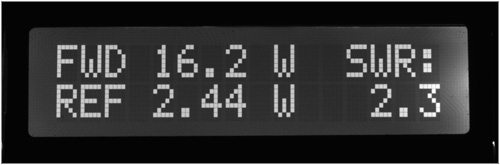
FIGURE 14-1 One of four display modes of the Directional Coupler/SWR Indicator.
SWR and How It Is Measured
Standing Wave Ratio, or SWR, is a measurement of the impedance match between a source and a load, in our case, a transmitter and an antenna system, and is expressed as a ratio, that is, “1.5:1 SWR” (read as “one point five to one”). We use the term system here because the load is comprised of much more than just the antenna. The load consists of the antenna, of course, but also includes the feedline and possibly an impedance matching network (i.e., an antenna tuner), connectors, switches, and the other components that comprise the actual load seen by the transmitter. To fully discuss the details of SWR is beyond the scope of this chapter. There are many good resources on the Internet and through various publications. A search on Wikipedia turns up an excellent discussion of SWR (http://en.wikipedia.org/wiki/Standing_wave_ratio). Simply stated, SWR is the ratio between the forward traveling wave on the feedline and the reflected traveling wave, the latter coming from any mismatch in the system.
Obtaining the Antenna System SWR
There are a number of ways to determine SWR either as the Voltage SWR or VSWR, or by measuring the forward and reflected power in the signal and deriving the SWR from their ratio. The measurement of RF power is a useful tool in troubleshooting and testing transmitters. Knowing both the SWR and the forward and reflected power is very useful as a measure of how well an antenna system is performing. There are many commercially manufactured SWR and Watt meters in the amateur market, but we chose to build one using an Arduino. There are a number of reasons we chose to build: 1) because we always like building things from scratch and maybe learning something in the process, 2) the design is tailorable to different applications, and 3) it’s often less expensive to build your own equipment. For this project we targeted the QRP community by limiting the meter’s maximum power handling to 20 W. However, we provide details on how to modify the design to increase the maximum power handling capability.
The SWR value is derived by measuring the forward and reflected power on the transmission line in our system. We use a very clever device called a “Stockton Bridge,” named after David Stockton, G4NZQ, the chap who first came up with this configuration for a directional coupler. A typical directional coupler is depicted in Figure 14-2 as a 4-Port “Black Box.” We refer to the depiction as a “Black Box” because describing the mechanism by which it works is beyond the scope of this chapter. However, we are able to accurately describe the coupler’s behavior. If you are interested in learning more about directional couplers, the Web is a good source. For the sake of brevity, we refer to the Stockton Directional Coupler as merely the “coupler.”
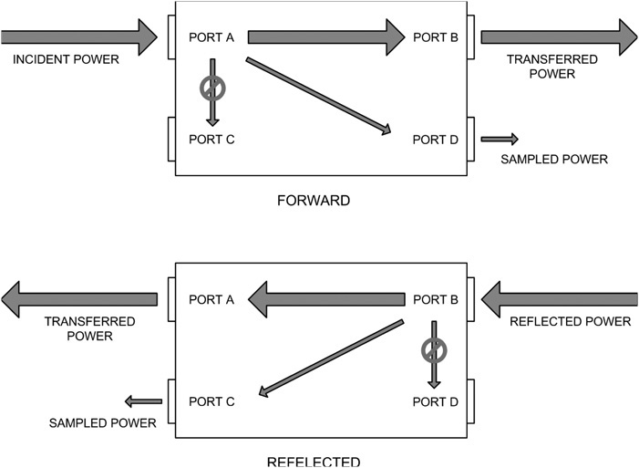
FIGURE 14-2 The Stockton Directional Coupler as a 4-Port Black Box.
Looking at the “FORWARD” drawing in Figure 14-2, a small portion of the power entering Port A is redirected to Port D while the majority of the power is passed through to Port B. At the same time, Port C receives virtually none of the power entering Port A. The coupler is also symmetrical. If we turn the coupler around and use Port B as the input, as depicted in the “REFLECTED” drawing, most of the power entering Port B is passed through to Port A while a small portion of the power is redirected to Port C, and Port D receives none of the power entering Port B. The ratio of the input power either on Port A or B with respect to the “sampling” ports (Port D and C, respectively) is called the “coupling factor.” The reduction in power between Ports A and B because of a small portion of the power being redirected is called “insertion loss.” And while the actual level is very small, the amount of power redirected between Port A and C or Port B and D is known as “isolation.” A fourth factor, “directivity,” is the difference between the coupling factor and isolation of Port C or D. We refer to Ports C and D as the sampling ports.
It should be apparent now that the coupler we have described could be a useful device for measuring forward and reflected power. With an unknown power level applied to Port A from a transmitter, and knowing the coupling factor, we measure the power at Port D and calculate the input power at Port A. In a similar manner, we measure the power at Port C and determine the reflected power from the antenna system. From this we calculate the SWR using the following formula:

where PF is the measured forward power and PR is the measured reflected power.
The four factors: 1) isolation, 2) coupling factor, 3) insertion loss, and 4) directivity, all play a part in how well the coupler performs. We want to minimize insertion loss and maximize isolation while setting the coupling factor such that we have a useful output for measurement. Reducing the coupling factor means that more of the input power appears on the sampling port, which increases the insertion loss. Poor directivity means that a portion of the reflected power appears on the forward sampling port. Coupler design becomes a trade-off of the four factors.
We have designed our coupler with a nominal coupling factor of 30 dB, meaning that 1/1000 of the power on the input ports appears at the sampling ports. The sampled power level using 30 dB of coupling factor is still sufficient that we are able to measure the power level without difficulty. The insertion loss is approximately equal to the input power minus the amount appearing on the sampling port; in other words, it is negligible. We want the isolation to be high in order to maintain directivity. Lowering the directivity means that errors are introduced into the measurements at the sampling ports. We maintain high isolation (therefore directivity) through careful construction of the components we use and proper shielding to eliminate stray signals. While all four factors are frequency sensitive, isolation and directivity tend to become worse as the frequency increases because of stray coupling in the coupler. This limits the useful frequency range to roughly 1 to 60 MHz.
Detectors
Most inexpensive SWR meters use diodes as their detectors. There are drawbacks to using a diode detector. First, a diode is not going to be sensitive to low power levels encountered with QRP operation. Second, at low voltage values diodes are exceedingly nonlinear, meaning that over the range of the meter using diode detectors, it is more difficult to measure and display low power levels. To mitigate the drawbacks of the diode detector, we use an active device in our design: a logarithmic amplifier made by Analog Devices, the AD8307. As the input voltage to the AD8307 varies exponentially over multiple decades, the output voltage remains linear. The AD8307, having a dynamic range of up to 90 dB, allows us to detect very low power levels while still being able to manage higher, as well as lower, power levels.
Constructing the Directional Watt/SWR Meter
This project is a little more complex than any we have attempted up until now. Our directional Watt/SWR meter consists of three components assembled into two major parts: 1) the remote sensor (a directional coupler with an internal detector), 2) the display unit (an interface shield with two op-amp DC amplifiers), and 3) an LCD shield. The software and hardware are designed to use either the LCD shield from Chapter 3 or an alternative design shown in this chapter that includes an RGB backlit display. Using the RGB backlit display offers certain advantages that we detail later in the chapter. The components of the SWR/Wattmeter are shown in Figure 14-3 along with the interconnecting cables, identifying the jack and plug designations. The remote sensor contains the directional coupler and the two log amplifiers. The display assembly contains the Arduino, an interface shield, and the LCD shield.
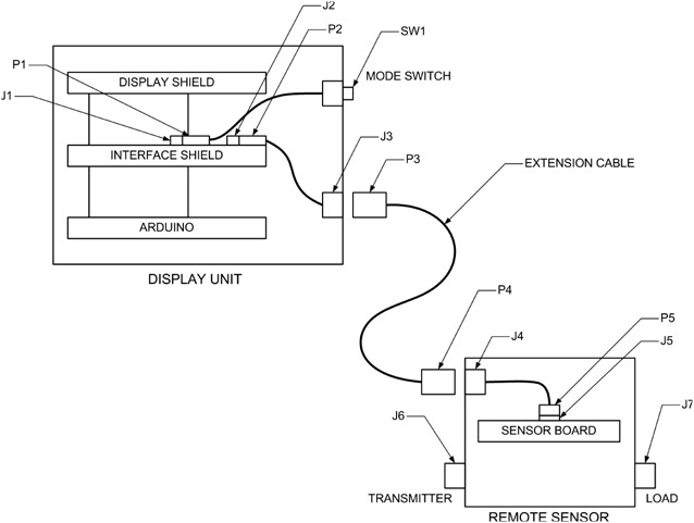
FIGURE 14-3 Components of the SWR/Wattmeter.
Construction of each of the components is described in the following sections. The overall parts list for the project is shown in Table 14-1.


TABLE 14-1 SWR/Directional Wattmeter Parts List
Design and Construction of the Directional Coupler/Remote Sensor
Figure 14-4 shows the coupler/sensor design schematic. The directional coupler consists of two identical transformers, T1 and T2, with 50 Ω terminating resistors, R1 and R2. R1 and R2 reflect the characteristic impedance of the system transmission line. We chose 50 Ω as this is the most common type of coaxial cable used in amateur antenna systems. If your system uses a different impedance, the values of R1 and R2 should be adjusted accordingly.
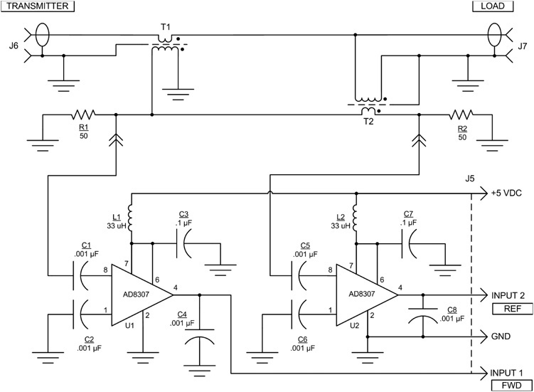
FIGURE 14-4 Schematic of the directional coupler and sensor.
U1 and U2 are AD8307 log amplifiers and they form the detector portion of our design. The AD8307 has a maximum input power of 15 dBm. Combining this with the coupling factor of 30 dB, the maximum permissible input power to the coupler is 15 dBm plus 30 dB or 45 dBm. This is roughly 20 W. If you wish to measure higher power levels, an attenuator must be used in front of pin 8 of the detector. Remember that the attenuator must reflect the characteristic impedance of the transmission line in the system. In the case of our system, the attenuator would have an input impedance of 50 Ω.
Our directional coupler/sensor assembly is housed in an LMB “Tite-Fit” chassis, Number 780, available from Alltronics in Santa Clara, CA (www.alltronics.com) or from Mouser Electronics in Mansfield, TX (www.mouser.com). The cost from either supplier is roughly the same, around $7.50 plus shipping and applicable taxes and shipping. The general layout of the coupler is shown in Figure 14-5.

FIGURE 14-5 Directional coupler chassis layout.
Figure 14-6 shows how the holes for the coax connectors and interface cable connector were placed on the ends of the chassis. We used a ⅝-in. Greenlee chassis punch to make the holes for the connectors. An alternative to a chassis punch is a ⅝-in. twist drill or a stepped drill, but the chassis must be very securely held down to prevent the drill from “walking.” A good technique for drilling holes in a chassis like this is to make up a paper template and tape it to the chassis. Punch the drill locations using a center punch and then remove the paper.
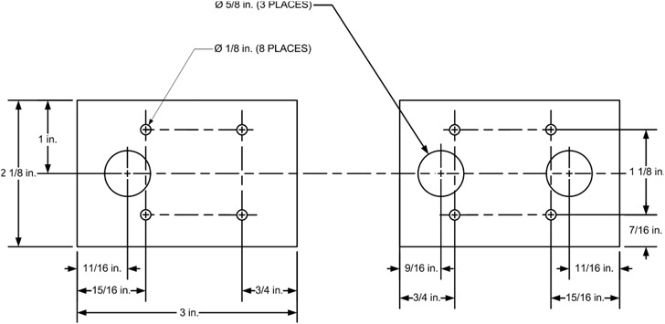
FIGURE 14-6 Chassis drilling dimensions.
The coupler uses two lengths of RG-8X. Cut the coax into two identical pieces per the dimensions as shown in Figure 14-7. The shield braid is exposed at one end only. Take a 3-in. piece of hookup wire and make three wraps around the exposed braid on the coax and then solder the connection. Transformers T1 and T2 are each wound on an Amidon FT-50-67 Ferrite core. The ferrite cores are available from Alltronics. Alternatively, the ferrite cores are available directly from Amidon (www.amidon.com).

FIGURE 14-7 Preparing the coax for the coupler.
Cut a 3-ft length of AWG24 enamel coated wire. Tightly wind 32 turns on the ferrite cores and then twist the free ends of the enameled wire together. Each time you pass the wire through the core counts as one turn. Spread the windings out as evenly as possible. The completed transformers should look like Figure 14-8. Slip one core over each the two coax pieces you have prepared. It takes some pressure to push the core over the coax as it is a tight fit. The finished transformer core and coax should look like Figure 14-8.
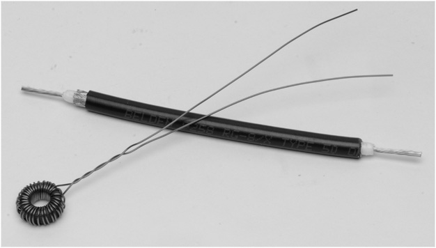
FIGURE 14-8 Ferrite cores after winding and the coaxial transformer.
The coupler includes two shields made from copperclad circuit board that are cut to 5 in. by 1½ in. We used this material because it is convenient to work with, but you might use other materials such as aluminum. The shields are shown in Figure 14-5 separating the two pieces of coax and the sensor board. Make sure, if you use doubled-sided copperclad board, that the two sides are connected together. We wrapped small wires around the edges and soldered them in place. Not having both sides connected did cause some confusing results early in the build. Floating grounds are not a good thing around RF.
A drilling guide is shown in Figure 14-9. Drill holes in one shield to allow the wires from the transformer cores to pass through to the next “compartment.” We used Teflon tubing to insulate the wires from the shield. Drill holes in the second shield to mount the sensor board (where the holes are placed depends on the choice of prototyping board used for the sensor board). Drill two mounting holes for the insulated standoffs used to hold the second coax assembly. We used a Cambion part for our coupler but these standoffs are difficult to find. We found ours on eBay. An alternative is to use a 4-40 thread, ⅜-in. insulated standoff with two solderlugs to attach the coax and to provide mounting points for the 50 Ω terminating resistors, R1 and R2. We used two 100 Ω ½ W carbon composition resistors in parallel for each of R1 and R2. The resistors we used came from Antique Electronics Supply located in Tempe, Arizona (www.tubesandmore.com). Resistors R1 and R2 are soldered to the copperclad board for grounding as shown in Figure 14-5. While it is not essential that these be carbon comp resistors, they must be noninductive. Carbon film resistors tend to be noninductive. Metal oxide and metal film resistors are trimmed with a laser-cut spiral making them highly inductive.
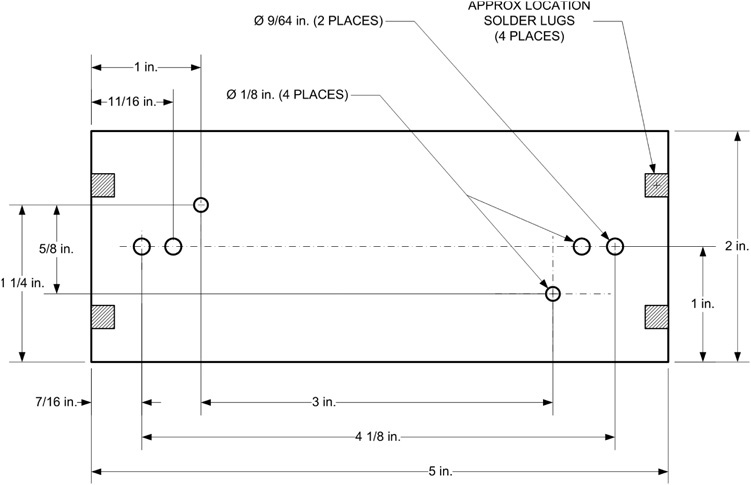
FIGURE 14-9 Drilling guide for the shields.
The Sensor Board
The layout of the sensor board is shown in Figure 14-10. The AD8307 is a surface mount 8-pin SOIC (“SOIC” is the acronym given to the “Small Outline Integrated Circuit” surface mount parts). The 8-pin SOIC is sometimes called an “SOIC-8” part. While the SOIC-8 part is very small, the truth is that it is much easier to work with than you might think. We used an SOIC-8 carrier to hold the AD8307. The bare carrier board and mounted AD8307 are shown in Figure 14-11. We obtained the carrier board from eBay by searching for “SOIC-8 carrier board.”
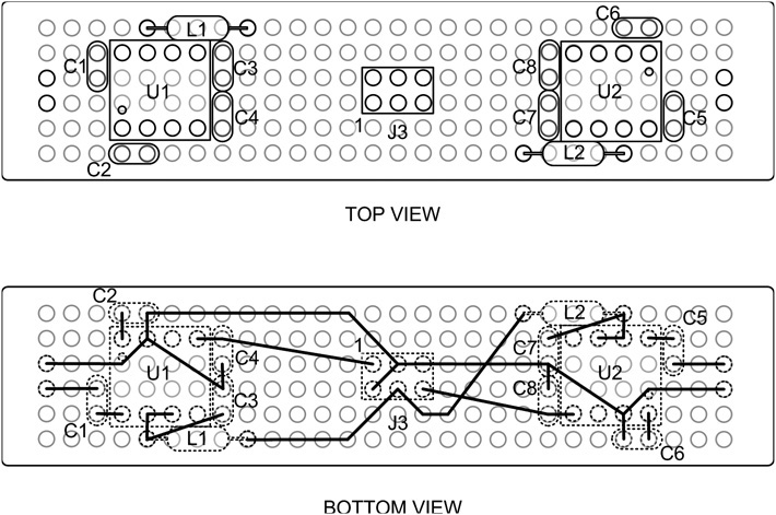
FIGURE 14-10 Sensor board layout and wiring.
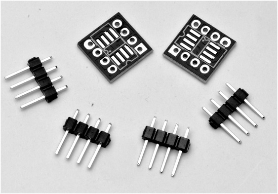
FIGURE 14-11 SOIC 8 carrier board and headers.
Soldering SOIC Components
Soldering the SOIC part to the carrier is easy if you follow the steps outlined below. Dennis has Dave Glawson, WA6CGR, to thank for teaching him this technique many, many years ago. Prior to Dave’s instruction, Dennis shied away from projects using surface mount parts (SMT). Today, he doesn’t give it a second thought. Hopefully, this technique is as beneficial to you as it was to him. Once you lose the fear of SMT, a whole new world of project possibilities opens up! There are two cautions though: 1) make sure that you have pin 1 on the SOIC package aligned with pin 1 on the carrier and 2) do not use excessive heat.
1. Apply a small amount of solder to one of the corner pads on the carrier (Figure 14-12). If you have some liquid flux, feel free to use it as well, but it is not essential.
2. Hold the SOIC part on the carrier and heat the pin you soldered in Step 1. A pair of tweezers is great for putting the part in place. A toothpick is a useful “tool” to hold the part in place (Figure 14-13).
3. Apply solder liberally to the remaining pins starting opposite the pin you just soldered in Step 2 (Figure 14-14). Be messy at this point. No need to overdo it, but don’t worry about solder bridges. We’ll fix them in the next step.
4. Remove the excess solder with solder wick (Figure 14-15).
5. Solder two 4-pin headers to the carrier (Figure 14-16). We use a solderless breadboard to hold the header pins while soldering.

FIGURE 14-12 Apply solder to one corner pad.
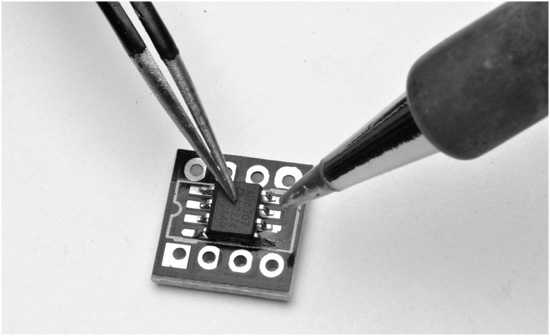
FIGURE 14-13 Apply the part and heat the pad you soldered.

FIGURE 14-14 Slather the pads with solder. You don’t need to be neat!
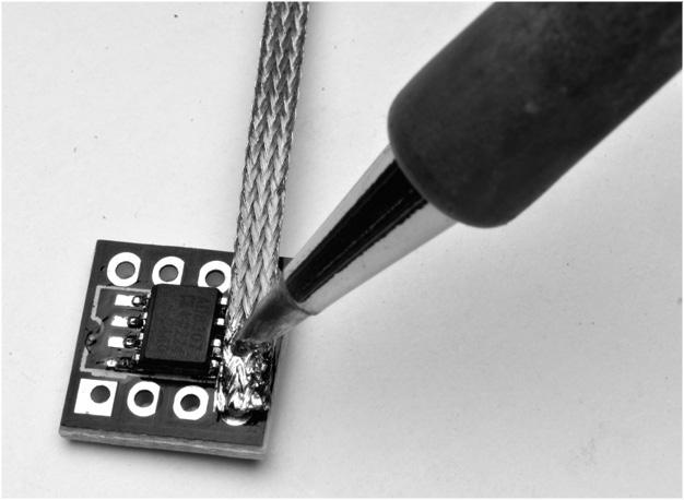
FIGURE 14-15 Remove the excess solder with solder wick.

FIGURE 14-16 Soldering the 4-pin headers to the carrier.
The finished carrier should look like Figure 14-17.
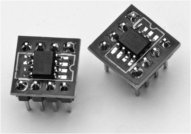
FIGURE 14-17 Voila! You just soldered your first SMT part!
Final Assembly of the Coupler/Sensor
Now it’s time to put the pieces of the directional coupler/sensor together. We mounted the copperclad shields to our chassis using solder lugs. The solder lugs were screwed to the chassis with 4-40 x ¼ in. machine screws and then soldered to the copperclad board. The wires from the transformers were passed through the holes in the shield separating the two pieces of coax and slipped through a short length of Teflon tubing. Be sure to observe the polarity of the windings; the wires must be attached exactly as shown in the schematic. Reversing a winding will actually do nothing more than reverse the Transmitter and Load ports, as well as the Forward and Reflected Power ports of the coupler. The sensor board should be mounted to its shield and wires routed through the shield to the standoff insulators holding the coax and terminating resistors using Teflon insulation over the wire to protect it from touching the shield. The ground wires from the sensor are soldered to the copperclad shield. We found that it was easier to mount the shields in the chassis before mounting the SO-239 connectors.
Make up a short jumper (about 4 in. in length) as shown in Figure 14-18 using six-conductor ribbon cable between the 4-pin mic connector and one of the 6-pin header plugs (FC-6P). The FC-6P connectors are easily found on eBay. They are also available as Harting part number 09185067803 from Mouser or Allied Electronics. We use a small vise to crimp the FC-type connectors onto the ribbon cable, but a pair of pliers also works. Be careful so as not to damage the connector. Regarding ribbon cable, scraps of ribbon cable are found in many places, most common being old computer disk drive cables. These tend to be 40 or 50 conductors, but it is easy to strip off as many conductors as you need using either a pair of flush cutters or an Exacto knife to separate the number of conductors you need from the rest. It is a simple matter of just “peeling” the six conductors away from the rest of the cable. Use an old pair of scissors to cut the cable to length.
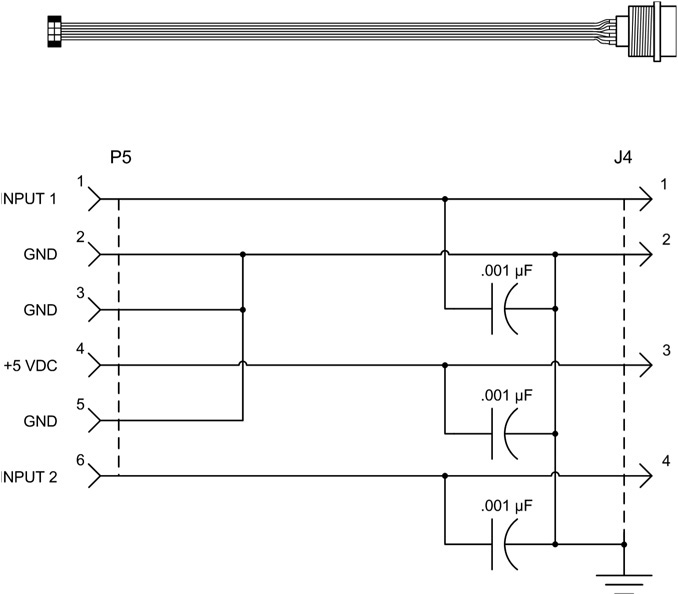
FIGURE 14-18 Sensor jumper cable.
Three 0.001 μF monolithic capacitors are used to bypass the power and sensor signal leads on the chassis connector. Solder one side of each capacitor to pins 1, 3, and 4 of the mic connector along with the six leads of the ribbon cable. We used a leftover solder lug from one of the SO-239 coax connectors as a tie-point for the ground leads of the capacitors. The FC-6P connector and ribbon cable are small enough to fit through the ⅝-in. mounting hole for the 4-pin mic connector. Do not solder the capacitors to the solder lug until the cable has been passed through the chassis and the mic connector is tightened down. When you attach the FC-6P connector to the sensor board be sure to observe the location of pin 1. Pin 1 on an FC connector is marked with a little triangle on one side near the end. A close-up of the coupler/sensor assembly is shown in Figure 14-19.
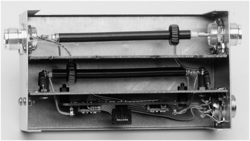
FIGURE 14-19 The completed directional coupler/sensor assembly.
Interface Shield Construction
The Interface Shield provides an easy way to not only connect the remote sensor to the Arduino, but it also provides some “level” adjustments to the output of each log amp on the sensor board. The interface shield is constructed using stackable headers so that the LCD shield is inserted on top. We used the circuit from the Chapter 5 panel meter with a few modifications. First, we don’t need the protection diodes across the input. Since this is permanently wired into a circuit, the diodes are not necessary. Second, we have adjusted the gain of the opamp to better suit the application, amplifying the output voltage of the AD8307A log amps. The maximum output voltage of the AD8307A is about 2.6 VDC (from the AD8307A datasheet). We adjust the 2.6 VDC to 3.6 VDC using the LM 324 opamp as a DC amplifier, just like in the panel meter. The gain required is Vout (3.6) divided by Vin (2.6) or about 1.4. Remember from Chapter 5 that the non-inverting gain of an opamp is 1 + RF/RG where RF is the feedback resistor and RG is the gain resistor between the inverting input and ground. Looking at Figure 14-20, the schematic of the interface shield, R5 and R6 form the feedback resistor for U1c and R4 is the gain resistor. In this application, we also remove the 51 Ω input resistor as would load down the output of the AD8307A. We leave a series resistor, R3, for the input from the sensor. The input resistance of the opamp is quite high, so the circuit does not load the output of AD8307 significantly.
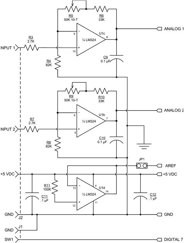
FIGURE 14-20 Schematic of the interface shield.
Just as we did in the Panel Meter design, we use one section of the LM324 opamp to provide the external reference voltage, AREF, for the Arduino analog to digital converter. U1d is configured as a voltage follower, driven to the maximum positive voltage by pulling up the non-inverting input to the positive supply rail through a 100 kΩ resistor. As a result, the output is the same as the maximum output of the two sensor amplifiers, U1b and U1c.
The interface shield was constructed using an Omega MCU Systems ProtoPro-B prototyping shield with the layout shown in Figure 14-21. If you use a different shield, the only thing you need to pay attention to is that you provide access to the adjustment potentiometers, R5 and R9. We show them mounted to the edge so that they are adjustable once the LCD shield is in place. Figure 14-22 shows the wiring side of the interface shield. The completed interface shield is shown in Figure 14-23 mounted on an Arduino Dumilanove.
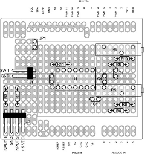
FIGURE 14-21 Interface shield layout.
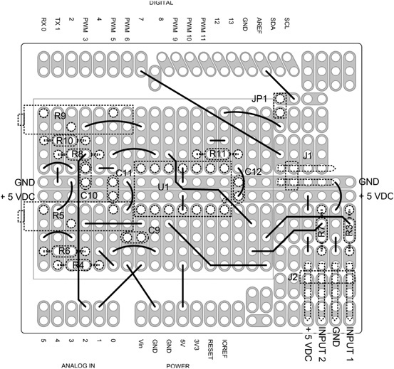
FIGURE 14-22 Interface shield wiring.
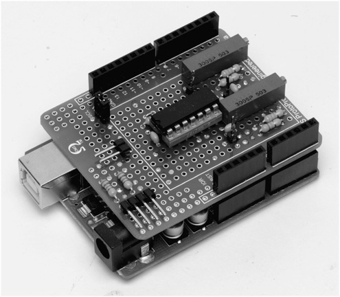
FIGURE 14-23 The completed interface shield mounted on the Arduino.
LCD Shield Options
While the LCD shield from Chapter 3 works just fine with our circuit, we decided to add a little feature by using an LCD with a multicolor backlight. We use the colors as a warning indicator as SWR is getting higher. White backlight means that everything is fine and that the SWR is within acceptable limits, usually below 2 to 1. As the SWR increases above 5:1 the display turns yellow. Above 10:1 it becomes red. The limits are all user-adjustable parameters set in software and are discussed in the software section of this chapter. The RGB LCD uses an 18-pin header. We added two additional resistors and along with the original 220 Ω resistor that was tied to ground, all three are now tied to digital output pins so that they may be turned on and off. Setting each of the three digital outputs (8, 9, and 10) LOW turns each of the three backlight LEDs on. Figure 14-24 shows the schematic of the new RGB LCD shield and Figure 14-25 shows the wiring side of the shield.
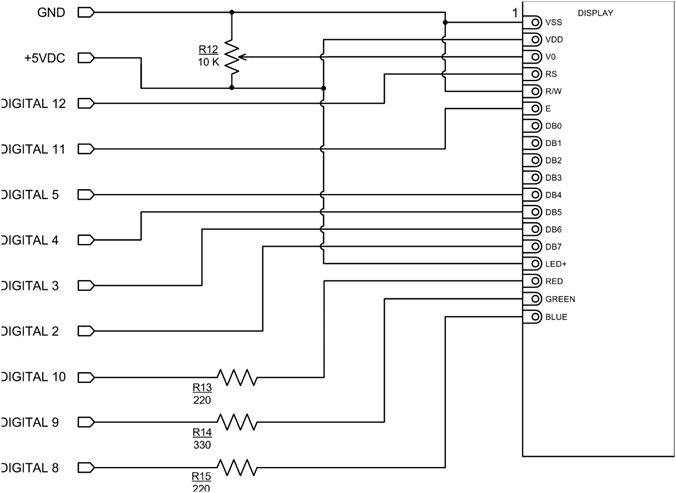
FIGURE 14-24 RGB LCD shield schematic.
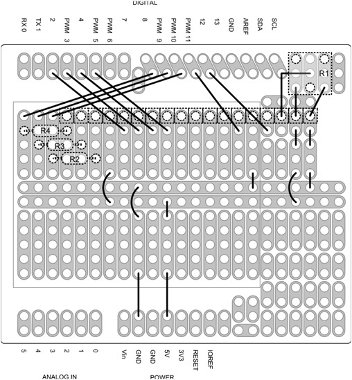
FIGURE 14-25 RGB LCD shield layout and wiring.
An easy way to make a quick check that your LCD shield is working correctly is to load the “Hello world” sketch from Chapter 3 and verify that the display is updating. However, the “Hello world” sketch does not activate the backlight LEDs.
Final Assembly
Now that you have completed the “heavy lifting” portion of the assembly, it is now time to bring it all together. The Arduino, display, and interface shields are mounted in an enclosure of your choice. We used an extruded Aluminum box from LMB; the same style as we used for the sequencer from Chapter 13. Refer back to Figure 14-3 for help identifying the various connectors and jumper cables.
We made two additional cables to connect the sensor to the interface shield. The first cable allows you to place the sensor remotely from the display. Use a cable length you feel appropriate to how you would like to place the sensor in relationship to the Arduino and display. Our cable is about six feet in length, uses four-conductor shielded wire, and has a 4-pin female mic connector at each end. The cable is wired pin for pin, or in other words, pin 1 is connected to pin 1 at the other end, pin 2 is connected to pin 2, and so on. The second cable connects a second chassis-mounted 4-pin mic connector to the interface shield inside the enclosure. The cable is shown in Figure 14-26 and shows the Molex connector, P2, pin positions.
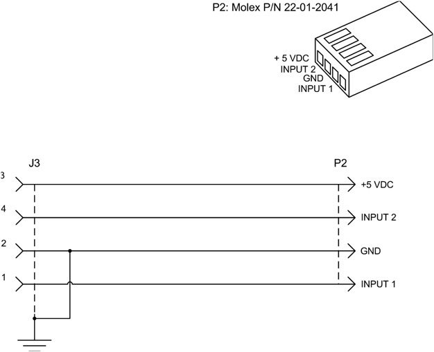
FIGURE 14-26 Display assembly jumper cable.
The completed pieces, the sensor assembly, interconnecting cable, and display unit, are shown in Figure 14-27. All that is left is to test the build by loading up the test software, and begin calibrating the meter! The listing for the test software is provided in Listing 14-1.
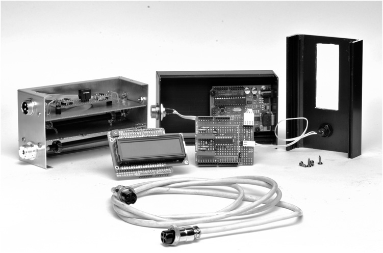
FIGURE 14-27 Completed components of the SWR/Wattmeter.
Testing the Directional Wattmeter/SWR Indicator
Testing and calibration requires a source RF between 25 and 50 W in the HF range. A modern HF transceiver with an adjustable output level is perfect. It is helpful if you have a known good Wattmeter as a reference. If you don’t have a suitable Wattmeter, look to borrow one from another local ham. Also, local high schools and community colleges may also be a source for you. Ideally, a dummy load with a built-in Wattmeter would be perfect (see Chapter 6 for the Dummy Load/Wattmeter).
Connect the RF source, dummy load, and directional coupler as shown in Figure 14-28. The dummy load must be capable of dissipating the 25 to 50 W we need for calibration, well within the limits of the dummy load described in Chapter 6. We use 50 Ω RG-8X jumpers or the equivalent for testing. Before connecting the pieces as shown, it is always a good idea to make sure that the cables, radio, and dummy load are functioning correctly. Connect the radio to the dummy load using each of the coax jumpers, testing them to make sure that they are making good connections. Bad cables lead to bad results.
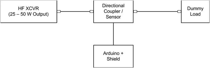
FIGURE 14-28 Test and calibration setup.
We used a simple program shown in Listing 14-1 to check that the sensors are working and that the Arduino is able to read the output of each of the log amplifiers, detect the switch, and change the LCD backlight colors. We also use this program to set the calibration points for use in the operating program shown in Listing 14-2. With a low power RF source attached as shown in Figure 14-28, apply power and observe the LCD display. As power increases, so do the values shown in the display. Pressing the pushbutton causes the LCD backlight to cycle through its colors. Once you have verified that things are working as they should, we calibrate the meter.
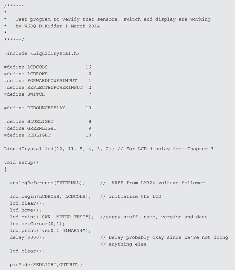
LISTING 14-1 Test software for the Directional Wattmeter/SWR Indicator.

LISTING 14-2 Arduino-based Directional Wattmeter/SWR Indicator.
Calibrating the Directional Wattmeter
Using the RF source as in Figure 14-25, set the output power to 20 W. The Wattmeter included with the Dummy Load in Chapter 6 is perfect for measuring the power. After verifying that the power level is 20 W, adjust the potentiometer, R5, so that the upper line of the display indicates a value of 1000. This is our first calibration point for forward power sensor. We know that 20 W input produces a count of 1000. We need one additional point to complete the calibration of the forward sensor. To ensure the accuracy of the Directional Wattmeter, the greater the difference between our calibration points, the better. We chose a power level of 20 mW for the second calibration point. However, we had the ability to accurately measure the power at that level using our HP 438 Power Meter. Record the results of the measurement. Make the second power measurement at as low a power level as you are able that is still within the range of the Directional Wattmeter. In other words, it should be greater than 100 μW. Again, record your results. Make sure that you record the power level you are using and the result displayed on the LCD.
The next step is to reverse the connections and calibrate the reflected power sensor. Repeat the two measurements, adjusting the reflected power calibration potentiometer, R9, for a reading of 1000 with 20 W input. Reduce the power and make a second measurement. The recorded values are used in the operating program for the Directional Wattmeter. You should now have eight values recorded: the high and low power settings in the forward direction and their corresponding analog output value, as well as those for the reflected direction. The next step is to edit the operating software with the measured calibration values and start using your new Directional Wattmeter/SWR Indicator.
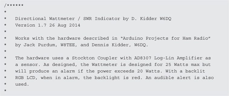
Software Walk-Through
The software for the SWR/Wattmeter is shown in Listing 14-2. For the most part, this program is straightforward and using the techniques we have been describing throughout the book. However, there are several new items that we discuss in more detail. What is important to know from this section are the definitions that are used to tailor the software to your build. Variations in component values result in different readings in the meter, hence the need for the calibration values that were recorded previously. The software uses the calibration data to set constants used to adjust the calculations so that the readings are correct.
Definitions and Variables
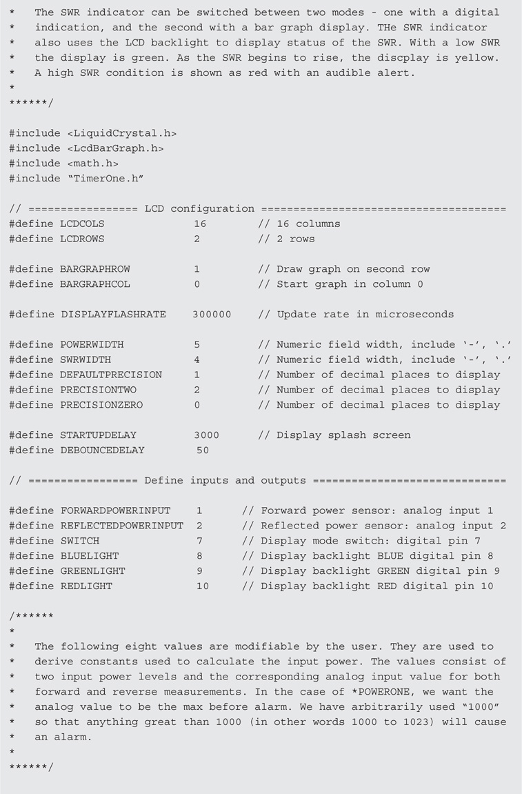
We begin with several #include compiler directives; Liquid.Crystal.h for LCD support, LcdBarGraph.h to generate a bar graph display as we did for the panel meter in Chapter 5, and two new libraries, math.h and timerOne.h. The math.h library is part of the Arduino distribution and provides a logarithm function needed for calculating RF power using a log amp. The timerOne.h library provides a timer interrupt function that we use. The timerOne.h library is downloaded from http://code.google.com/p/arduino-timerone/downloads/list.
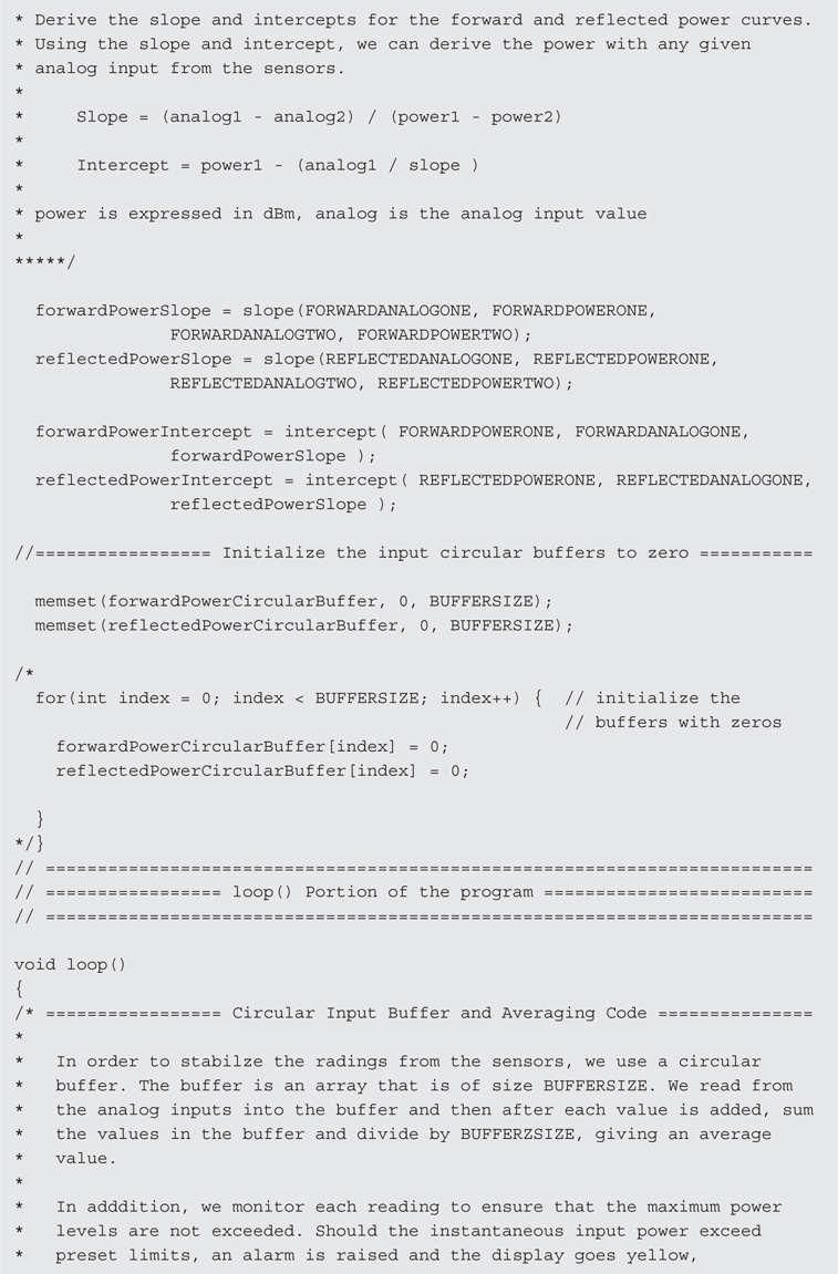
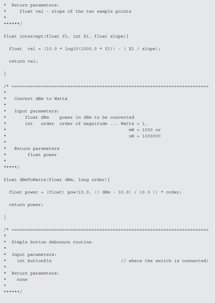
The set of definitions starting with FORWARDPOWERONE are modified by the user to calibrate the power meter. As you know, the log amp measures power over a logarithmic scale and produces an output voltage that is the log of the input power. In order to convert to the equivalent power read from the input power read, we use a little bit of geometry, creating a line (representing the input power versus output voltage) with a slope and an intercept. Knowing the slope and intercept of the line, we are able to calculate the input power for any output voltage.
During the checkout and calibration procedure you captured two data points for each of the two sensors, forward and reflected. The calibration values are substituted into the eight #define statements as shown. The comments indicate which value goes where. The power values are the input RF power and the analog values are what was recorded form the LCD screen. The values included in the listing are for the sensor we built. The program uses these values to determine the slope and intercept for the forward and reflected power conversion.
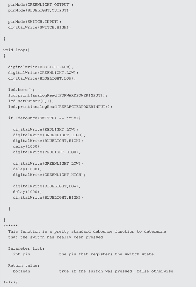
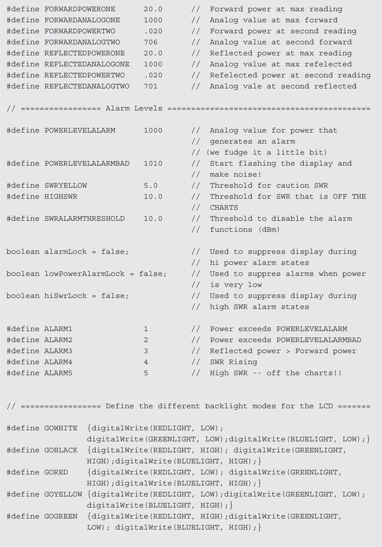
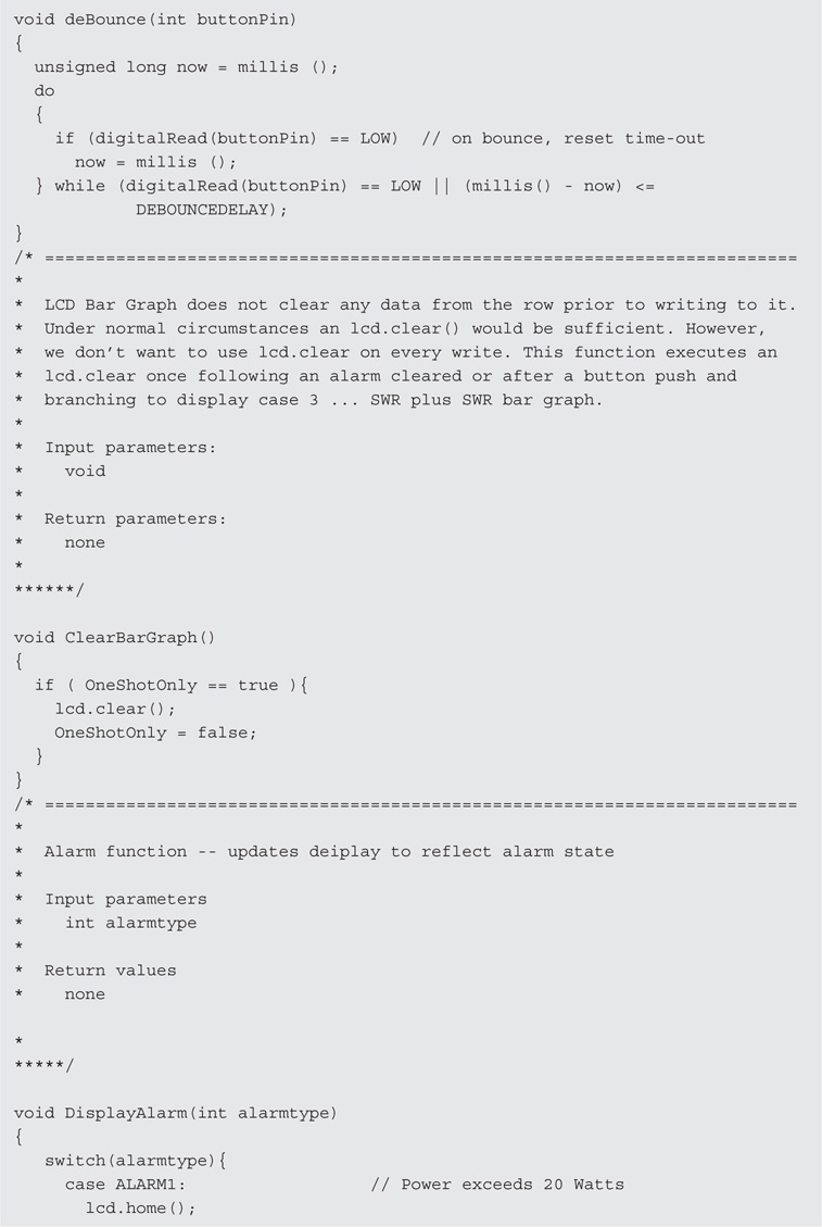
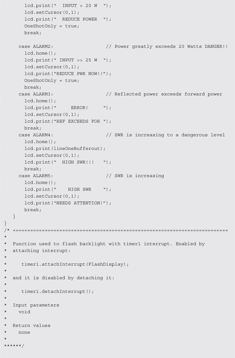
The Wattmeter/SWR Indicator also includes several useful alarm functions. The alarm functions warm the operator of potentially harmful conditions such as high SWR or excessive power. High SWR can damage transmitting equipment so it is a good idea to avoid this as often as possible. Excessive power, on the other hand, can damage the power sensors in the directional coupler. The Alarm level section contains the threshold values for excessive power and SWR. The power alarm is of two stages, meaning that there is a “nudge” warning as you approach the dangerous power level, changing the color of the display backlight to yellow. The second stage is more insistent by flashing the display with a red backlight. If you should desire to do so, it is a simple matter to add an audible warning as well by adding another digital pin as an output to drive a buzzer.
We use a series of macro definitions provide a simple way of executing repetitive sequences of commands with a single name. What we have done is defined a series of digitalWrite() commands to set the different backlight colors. This macro definition:
![]()
creates GOWHITE that may be used anywhere in the program where we wish to set the backlight to white. Note the braces that surround the macro definition. In order to flash the red backlight, we use a timer interrupt and set the timer delay to the value defined by DISPLAYFLASHRATE.
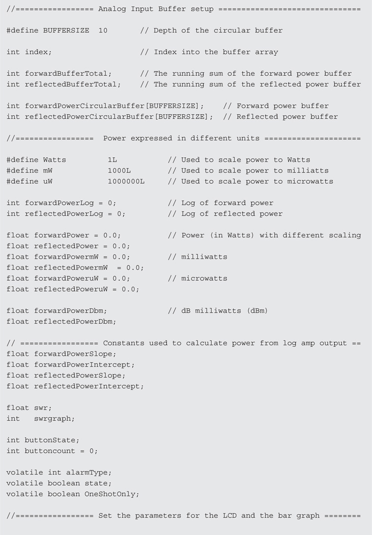
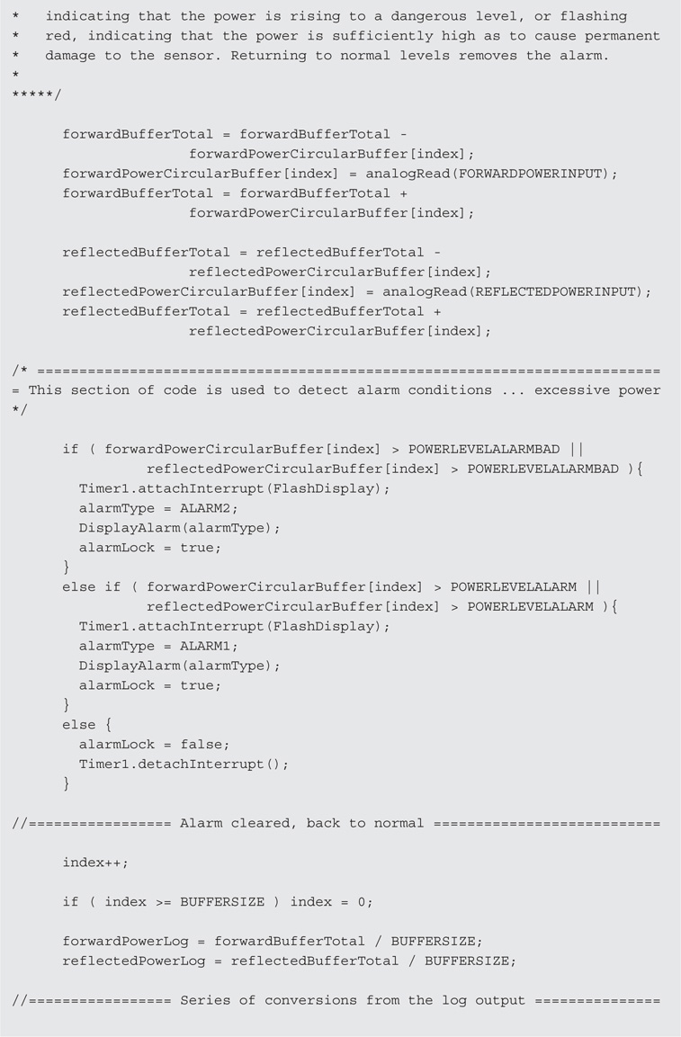
One trait of the Arduino analog input functions is that, with any given analog input, there is more than likely going to be some jitter in the output values. This is not unusual for an analog to digital converter. In order to provide a more stable display, we decided to average a number of consecutive readings, thus smoothing the values being displayed. This is also called “smoothing.” To average the values we set up two arrays: forwardPowerCircularBuffer and reflectedPowerCircularBuffer. As the name implies, these are “circular buffers,” a fixed length buffer that is connected end-to-end, giving the appearance of an endless buffer. The key here is that with a buffer length of “n,” the “n+1th” entry overwrites the “0th” entry. We then take the sum of the entries and divide by “n,” the result being the average of the last “n” values. BUFFERSIZE sets the value of n.
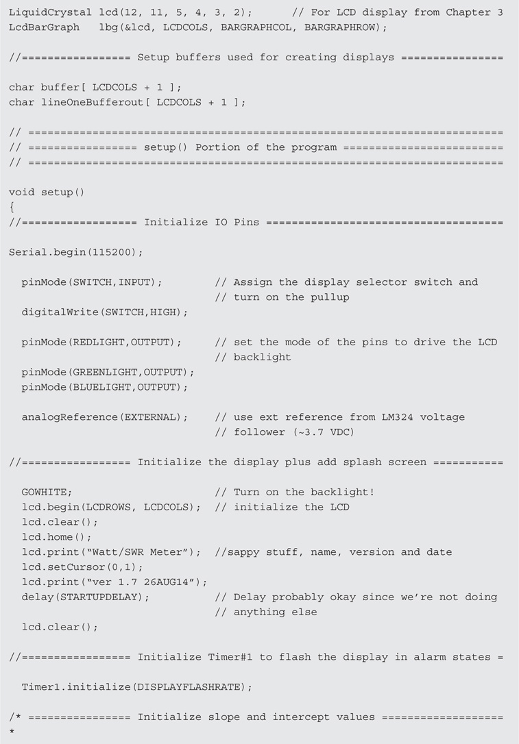
setup()
Within setup() we initialize the input and output pins, the LCD and set the contents of the circular buffers to “0.” To initialize the buffers, we use the memset() function:
memset(forwardPowerCircularBuffer, 0, BUFFERSIZE);
to set the contents of the arrays to zero. The memset() function is a standard library function that is tweaked for efficient setting of memory blocks to a given value. In addition, we calculate the calibration constants for slope and intercept from the calibration values edited from the test results.
Recall that we are using a circuit similar to that of the panel meter from Chapter 5. In this case as in Chapter 5, the op amp is used as a DC amplifier to scale the voltage from the log amp to a range more compatible with the analog input pins of the Arduino. In Chapter 5, we discussed the need to use an external voltage reference for the analog to digital converter (ADC). We have used the same design here, using one section of the quad op amp to provide the external reference voltage for the ADC. Remember that you must have executed the analogReference(EXTERNAL) command prior to connecting your interface shield to the Arduino. Just as in Chapter 5, there is a risk to the Arduino processor when the internal and external references are connected at the same time. To make things easier, we include a jumper pin on our shield to disconnect AREF if it is needed. It’s much easier to pull the jumper than disassemble the stack of cards.
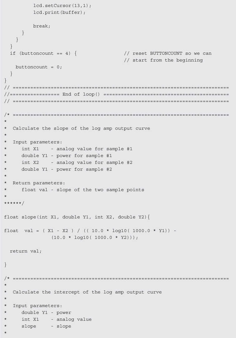
To determine the slope and intercept, we use two values of power and voltage for each of the two sensors. The slope is derived by the following equation, taken from the AD8307 datasheet:
slope = (analog 1 – analog 2)/(power 1 – power 2)
where analog 1 and analog 2 are the output of the ADC for the corresponding input power levels, power 1 and power 2. The equation for determining the intercept also comes from the AD8307 datasheet and thus:
intercept = power 1 – (analog 1/slope)
where power 1 and analog 1 are as used by the slope equation and slope being the result of the slope calculation.
loop()
The loop() section of the program is where the input and output processing takes place. We break loop() down in to a series of functions that, in sequence, read the raw data from the sensor, perform conversions between the value read and the values to be presented as output, and lastly, format the output data and send it to the display.
The first thing we do in loop() is read the analog inputs from the two sensors and average them using the circular buffer. The following snippet of code illustrates the code for the forward power sensor:

The variable, forwardBufferTotal, is the sum of the values in the buffer. The first thing we do is subtract the forwardPowerCircularBuffer[index] value from the total. We then read the analog input and load the result into the array at index, and then add the value to forwardBufferTotal. We then increment index, and if it is greater than or equal to BUFFERSIZE it is reset to zero. The total is then averaged by diving by BUFFERSIZE. The remainder of loop() is processed and the sequence is repeated.
The circular buffer code also contains tests for the high power alarms. As the buffering and averaging produce some delay, we decided that it would be a good idea to detect high power and raise the alarm as quickly as possible. Rather than waiting for the average value, we alarm on the instantaneous value of each sensor. In other words, we test each reading to see that they are in the safe range. The following is the power alarm detection:
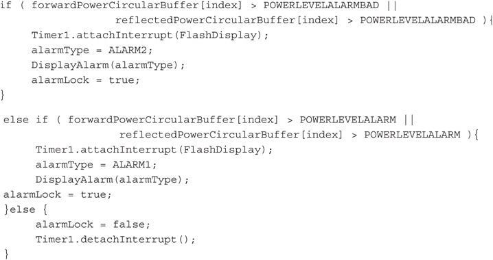
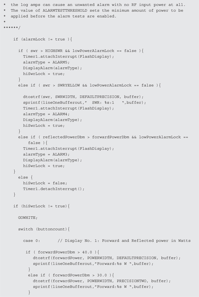
The tests for high power are made against the raw, analog value, rather than going through the conversion process. Since 20 W is represented by an analog value of 1000, anything over 1000 is considered an alarm. An analog reading of 1010 is roughly 25 W and that is our second threshold for alarming. Above 20 W, the display changes to a yellow backlight. Above 25 W the display changes to a flashing red backlight. We use an interrupt from timer1 to flash the red backlight on and off.
One way to flash the display backlight is to use a delay() statement, but delay() has some negative effects on programs, primarily, when the delay() is executing the processor is not able to do any other processing, including interrupts. Rather than using delay() statements, we opted to use an interrupt set by timer1 and use the interrupt to turn the red backlight on and off. We set timer1 to generate an interrupt after 300,000 μS have elapsed. The statement:
Timer1.attachInterrupt(FlashDisplay);
is used to “attach” the timer to the function FlashDisplay(), in a sense, enabling the interrupt. The timer is first initialized in setup() with:
Timer1.initialize(DISPLAYFLASHRATE);
setting the timer’s overflow value at DISPLAYFLASHRATE, or 300,000 μS. Once the timer interrupt is enabled, the overflow causes an interrupt to occur every 0.3 seconds, invoking the function, FlashDisplay(). The function sets the backlight color and depending on the alarm, flashes the backlight.
The boolean, alarmLock, is used to lockout additional display processing during an alarm condition. When there is an alarm condition, alarmLock is set to true. When the alarm condition is cleared, alarmLock is set back to false.
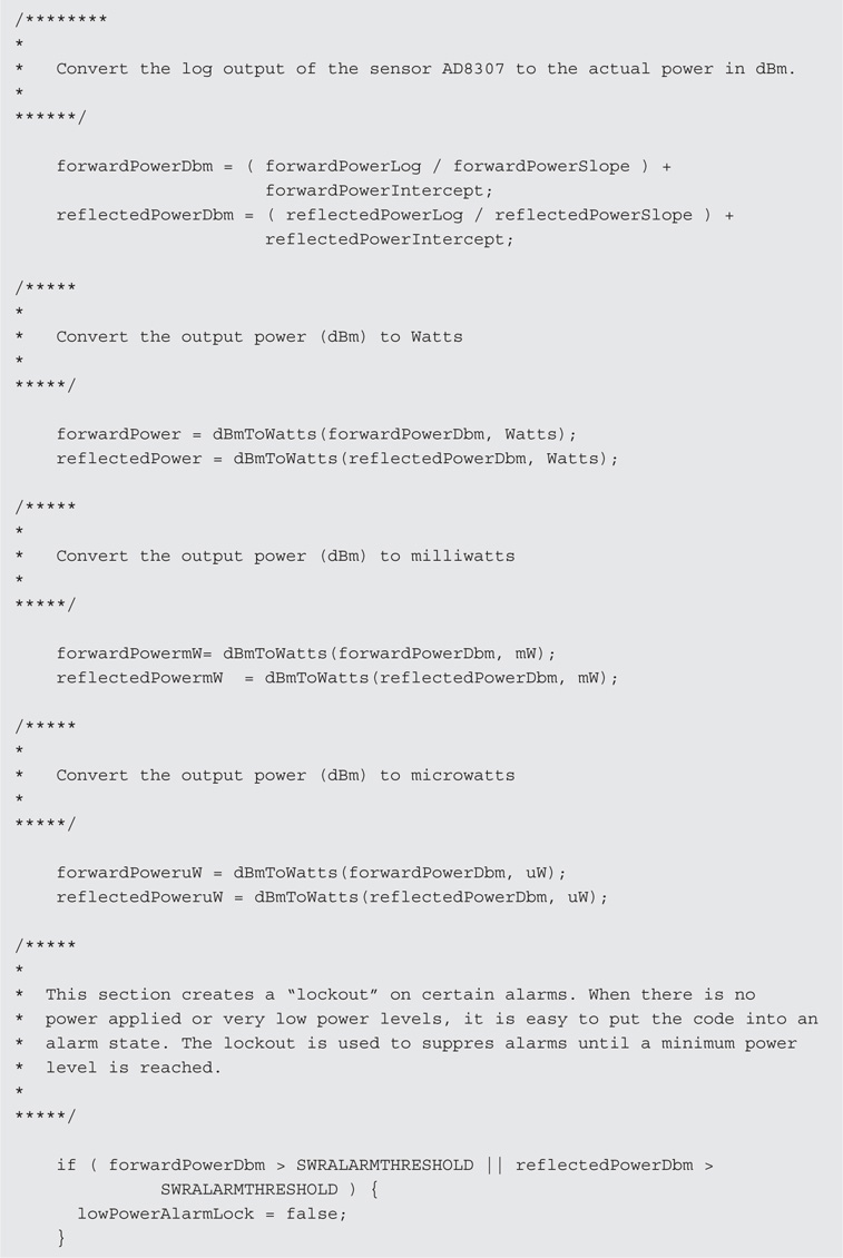
All of our power measurements from the AD8307 are a voltage representing the power expressed in dBm or “decibels milliwatt.” Since power is a logarithmic function, dBm provides a linear progression through decades of power levels. The value “0 dBm” is equal to 1 mW. Therefore, 10 mW would be 10 dBm, 100 mW would be 20 dBm, and 100 μW would be –10 dBm. By converting the analog input value to dBm, the measured power may be displayed in Watts, milliwatts, microwatts, and of course, dBm. We again use a little geometry to calculate the power in dBm from the input analog value. Recall that in setup() we derived a slope and intercept for each sensor? Now it’s time to use those values to calculate the power. We use the equation:
Power (in dBm) = (analog input/slope) + intercept
where slope and intercept are the values calculated in setup() for the sensors. The result is expressed in dBm.
It is now a simple matter to convert from dBm to power in Watts. The equation:
Power (in Watts) = 10 to the power (power in dBm – 30) / 10
Is used for the conversion. The code looks like this:
![]()
where we are using a new function pow(). The function pow() is used to raise a number to an exponent, in this case power in dBm minus 30 and then divided by 10 is an exponent of the base, 10.0. The resulting value is in Watts. Since 1 W is 1000 times 1 mW and 1 mW is 1000 times a μW, it becomes simple math to convert between these different units of measure.
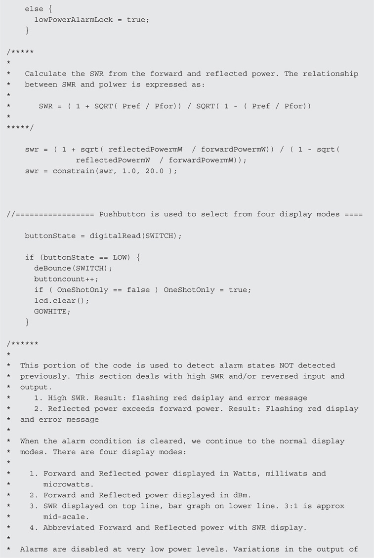
One of the major functions of the Wattmeter project is to provide an SWR reading. The next steps calculate SWR, using the power measurements as input. Recall from earlier that the formula for calculating SWR is:
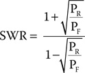
where PR is the reflected power and PF is the forward power.
Just as was done for excessive power levels, we test for high SWR and set alarms. As in the power alarms, the SWR alarms are set in two steps, the first being an SWR above 5:1, and the second, 10:1. Above 5:1, the backlight is set to yellow, and above 10:1, the backlight is set to red and flashed on and off using FlashDisplay().
The SWR alarms use two additional locks: highSwrLock and lowPowerAlarmLock. The first lock, highSwrLock, is used to stop additional display processing while the alarm is on the screen, just as we did with the high power alarms. The second lock, lowPowerAlarmLock, serves a slightly different purpose. If the reflected power is greater than the forward power, the resulting SWR is a negative value. Applying power with the coupler connected in reverse is one way that this happens. There are also situations where the apparent reflected power is greater than the forward power. Even with no power applied, it is possible to produce a negative SWR. With no power applied, the analog input values are the quiescent output voltage of the log amps.
Because of variations between parts, it is possible to have the reflected power log amp having a larger quiescent voltage output then the forward log amp, hence a negative SWR reading. Since we really don’t want to have an alarm when there is no power applied, lowPowerAlarmLock, prevents the SWR alarms from occurring below a preset power level, in this case 10 mW. The quiescent levels of the log amps with no input are typically in the 100 μW or –10 dBm range.
Last but not least, we format the power readings and SWR values to be sent to the display. Placing the decimal point becomes important when displaying data over many orders of magnitude range. Our meter directly measures power levels from less than 100 μW up to 20 W, over five orders of magnitude. In testing our meter in Dennis’s lab, we found that the measured values were typically within 5% of readings made with his Hewlett Packard Model 438 Power Meter. More often than not, they were in the 1 to 2% range of error. Understanding the accuracy of an instrument is important to formatting how the results are displayed. For instance, given an accuracy of 5%, we would not provide a display of 10.00 W because that last fractional digit would be ambiguous as it is significantly smaller than 5% of the total value. We would choose to display the results as 10.0 because 5% of 10.0 is 0.5 corresponding to one fractional decimal place in the display.
Thus we adjust the display format based on the order of magnitude of the reading. The first step prior to any display formatting is to test for excessive input power, excessive SWR of reversed forward and reflected connections. If there are no alarm conditions, we proceed to the display selection based on the number of times the input switch is pressed.
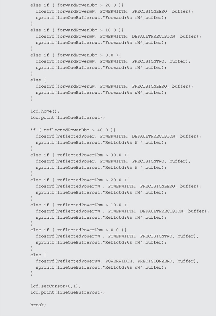
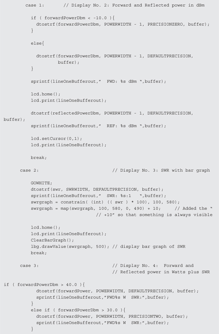
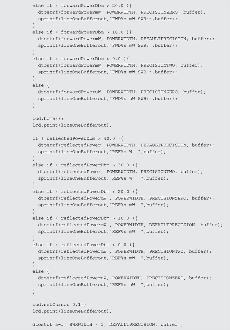
There are four possible display formats:
1. Forward and Reflected power in Watts, mW and uW.
2. Forward and Reflected power in dBm.
3. SWR displayed in addition to a bar graph.
4. Forward and Reflected power in Watts with SWR.
There is one known bug in the program. Repeatedly pressing the pushbutton cycles through the four display modes of the Directional Wattmeter. The first time through the displays, the SWR bar graph displays as expected. However, subsequent cycles bringing up the SWR bar graph do not display the bar graph unless the input values for either forward or reflected power change. In a practical sense, there is enough jitter and noise in the system such that this is not a big issue. A little bit of noise on the input and the display pops right up. It’s one of those items that just nags at a developer to make it right.
Further Enhancements to the Directional Wattmeter/SWR Indicator
The Directional Wattmeter was designed for QRP operation and has a limit on the amount of power that can be applied without damaging the sensor’s log amps. To measure higher power levels, it is a simple of matter of inserting an attenuator in front of the inputs to the log amps. The attenuator must be designed for the characteristic impedance of the line section, or in our case an input impedance of 50 Ω. The log amp itself represents a load of about 1000 Ω. Another consideration for high-power operation is the choice of ferrite cores in the sensor. The cores we have used become saturated at higher power levels, the result being that the higher power readings become nonlinear. The design for a higher power sensor requires larger ferrite cores, such as the Amidon FT-82-67, and rather than RG-8X, uses RG-8/U or the equivalent. The turns ratios remain the same; the higher-power cores have 32 turns just as the ones we made for this Wattmeter.
Conclusion
There is always room for improvement in any endeavor. This project is no exception. We leave it up to the user to create new display formats for the project. Maybe you would like to see two bar graphs indicating power or possibly even a four-line display. Feel free to exercise your creativity, but be sure and share your ideas and changes with us on our web site (http://www.arduinoforhamradio.com).