CHAPTER 5

A General Purpose Panel Meter

As we mentioned in Chapter 2, one important aspect of any μC system is to be able to display data. Panel meters are found in many “homebrew” projects. Any radio amateur who’s been around a while is bound to have a few old meters hanging around the workshop. We find them at the swap meets or remove them from some old piece of gear we’ve parted out. Chances are good, however, that the one you found in your junk box has unknown characteristics and a scale that needs to be replaced. Although replacing a scale is not too difficult—there is software available to print a new scale—you run the risk of damaging the delicate meter movement while swapping the scales.

This chapter’s project creates a general purpose panel meter that is designed to read 0–1 mA full scale. The project presents both digital and analog displays on the two-line LCD constructed in Chapter 3. Changing the range of the meter is easy using external resistors, and we provide examples of how this is done. Because the display is generated by software, it becomes trivial to change the displayed range; it’s just a text string. We also show a simple means of calibrating the meter so that it reads correctly. Figure 5-1 shows the meter in action.

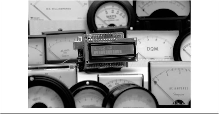
FIGURE 5-1 The general purpose panel meter in action.

 

Circuit Description

The panel meter is modeled after a typical D’Arsonval 1 mA meter. In this case, the meter presents approximately a 50 W load with 1 mA of current flowing. The actual value of the input resistor (R1 in Figure 5-2) is not critical, but it is needed to calculate any external scaling that is utilized. We used a value of 51 Ω in the current version. Ohm’s law tells you that 1 mA of current through a 50 Ω resistor produces a voltage of 50 mV. That 50 mV is then read by the Arduino analog input.

FIGURE 5-2 Schematic of the general purpose digital panel meter.

The analog input uses an analog-to-digital converter, or “ADC,” to represent the analog voltage as a digital value. The digital value is 10 bits in length or, to look at it in a different way, the analog input is represented by 1024 digital values (0000 through 1023). However, the input range of an Arduino analog pin is from 0 V to 5 VDC (5 VDC = 1023) and this presents a problem. Our voltage across the input resistor is only 50 mV. If 50 mV is fed to the ADC, the highest value from an analog read is 0010 and the accuracy and resolution of the incremental values would be very poor. We would be able to display only 11 discrete values. This would not be a very good panel meter.

Instead, we use an operational amplifier (op amp) (U1a in Figure 5-2) to amplify the DC input voltage to a higher value. We chose an LM324 op amp for this project. The LM324 is a quad op amp, meaning that there are four identical op amps in a single IC package. There are single op amps available, such as an LM741. However, we chose to go with the LM324 for several reasons. First, it operates off of a single voltage supply without additional biasing. Second, they are readily available and inexpensive, usually less than a $1 each. Third, we plan on adding some additional circuitry to the shield in future projects and will make use of those additional, unused, op amps later on.

Because the op amp is running on 5 VDC supplied by the Arduino, the maximum output voltage from the op amp is about 3.5 VDC—a function of the design of the op amp. While not perfect, the LM324 provides better range than a maximum input voltage of 50 mV. Resistors R2, R3, and R4 in Figure 5-2 set the gain of the op amp (GAIN = 1 + ((R3 + R4) / R2)). R3, a 10-turn potentiometer, provides the means to make fine adjustments to the gain of the amplifier. With the gain set to 70, we would have roughly 716 values giving us greater resolution of the meter’s input current.

 

NOTE: According to the LM324 datasheet, the maximum output voltage would be

VCC – 1.5 = 5 – 1.5 = 3.5

If we apply the GAIN formula using the values suggested in Figure 5-2, then:

GAIN = 1 + ((R3 + 270K) / 4.7K)

and the range of values for GAIN is a minimum of about 57 to a maximum of almost 79.

The bad news is that adding the op amp is still not optimum because we would like to have our maximum input provide a full count of 1023 in the ADC. However, the good news is that there is an easy cure! The Arduino includes a little feature on a pin called “AREF.” AREF, or “analog reference,” allows us to provide an external reference voltage to the ADC. The ADC samples the voltage present on the analog input pin using the analog reference for comparison. The voltage used as the analog reference represents the largest voltage that can be measured on the analog input. The Arduino defaults to the internal reference voltage of 5 VDC, which means that, in order to have a reading on the analog input of 1023 counts, we would need 5 VDC on the analog input. Because our op amp circuit can only produce about 3.5 VDC maximum, we can configure the Arduino to use an external reference, with 3.5 VDC applied to AREF, in order to obtain a count of 1023 when the op amp is producing the maximum output. So, how to produce 3.5 VDC?

One nice feature of using a quad op amp, such as the LM324, is that not only are they in the same package, all four devices share the same substrate material on the integrated circuit die; therefore, their electrical characteristics tend to be almost identical. We can take advantage of this “feature” to create a voltage of 3.5 VDC to use as the external analog reference. With an unused section of the LM324, we create a 3.5 VDC reference by configuring the op amp as a voltage follower (a non-inverting amplifier with unity gain) and pull the non-inverting input to the positive voltage rail. With 5 VDC on the non-inverting input, the output of the op amp is 3.5 VDC and the same as the maximum voltage that is produced by the DC amplified section of our circuit. Now when we apply the maximum input value to our meter circuit, the ADC provides a count of 1023 rather than 716 as we described earlier when using the internal reference.

Note how the output of the LM324 feeds into the AREF pin on the Arduino. This means that the AREF pin receives the 3.5 VDC, which serves as the internal reference voltage for the ADC circuit of the Arduino. The line in Listing 5-1 (presented toward the end of the chapter):

is responsible for establishing the reference voltage for the Arduino. Note that you can change the symbolic constant INTERNAL to EXTERNAL for debugging purposes without having to use the reference voltage. To use an external reference voltage on the AREF pin, you must call analogReference(EXTERNAL) before calling analogRead(). CAUTION: Do not apply less than 0 V or more than 5 V to the AREF pin, otherwise you might “brick” your Arduino. (The term “brick” means to transform your Arduino board from a useful electronic μC into a silicon brick.) You can use analogReference(INTERNAL) to generate “fake” analog readings (i.e., analogIn in Listing 5-1) for testing purposes. This proved helpful while the hardware was being built in California but the software was being written in Ohio!

As can be seen in Figure 5-2, section U1b of the LM324 is configured as a voltage follower with the non-inverting input connected to 5 V through a 100K resistor (R5), driving the output of the follower to the maximum voltage or about 3.5 VDC. A parts list for the panel meter is presented in Table 5-1.

TABLE 5-1 General Purpose Panel Meter Parts List

Another requirement of a digital panel meter is to indicate when the input value exceeds the maximum range. Unlike a mechanical panel meter whose indicator can move past the full-scale value (or becomes “pegged”), the digital panel meter reaches the full-scale value and goes no higher. It is the nature of a digital panel meter design that, as the input voltage increases above the 50 mV full-scale value, the displayed value does not increase. The op amp is “saturated” and can’t produce a higher output voltage for the ADC to read. Because the ADC can count to 1023, and we want to be able to detect the overrange condition, we arbitrarily set a count of 1000 to equate to 1 mA, giving us the range of 1001 through 1023 to indicate the overrange values. So, what we want is to have 1 mA input current equal to something less than count of 1023. The beauty of using the AREF input is that, if we set the gain of the op amp so that 1 mA input current equals a count of 1000, the output voltage is less than the maximum, giving us the extra “headroom” to detect the overrange values. Anything over 1000 and the meter is “pegged” and displays the overrange message.

Because the LM324 input has a maximum rating that cannot exceed the supply voltage or below ground, we have provided the 1N4001 diodes to provide protection for the op amp input circuits. The diodes do “clamp” the input voltage approximately 0.6 VDC above the positive supply voltage or 0.6 VDC below ground or 0 VDC. The diodes provide a margin of safety for the op amp.

To further improve the usefulness of the digital panel meter, an analog bar graph has been placed on the second line of the display. This tracks the input quickly and allows a nice indicator for fine adjustments you may be making, much like a conventional analog meter.

There is one drawback to this design and it is an important one to note. As it is constructed, one side of the meter input is connected to the negative lead (“ground”) of the power source. For applications as a voltmeter reading a positive voltage, this is no big deal. However, using the meter as an ammeter or to measure a negative voltage, the ground becomes an issue. The solution is to “float” the entire assembly above ground. One way to do this is to provide power through an isolated supply, such as a “wall wart.”

Later in the chapter we give instructions on how to change the meter from a milliammeter to a voltmeter or an ammeter, and how to change the unit’s value on the display.

 

Construction

The parts used for construction of the general purpose panel meter are shown in Figure 5-3. At the top left, the four ¼ W resistors; top center, the prototyping shield; to the right, a 14-pin DIP socket; and below the socket, the LM324 Quad op amp. Across the bottom from the left: R3, a 100K 10-turn pot; C1, a 0.1 μF monolithic capacitor; the two position screw terminal; and D1, D2, the 1N4001 diodes.

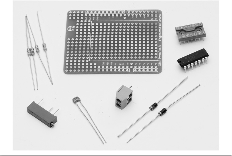
FIGURE 5-3 Parts used for the general purpose panel meter.

The panel meter shield is constructed on an Omega MCU Systems ProtoPro-B prototyping shield, the same shield used for the LCD shield and RTC/Timer projects. Figure 5-4 shows how we placed the parts on the shield. The LM324 op amp is mounted in a 14-pin DIP socket. It is much easier to solder wires to the socket rather than the leads of the IC package and it eliminates the possibility of damaging the IC with too much heat while soldering. The terminal connector block (or “screw terminal”) is used to make it easier to attach the panel meter to your circuit. The 10-turn pot should be mounted so that it can be accessed with the LCD shield or display installed, with the adjustment screw to the outside edge of the shield. You need to adjust the 10-turn pot while the panel meter is operating in order to calibrate the meter reading. (The calibration procedure is described in the section on testing and calibration of the meter.)

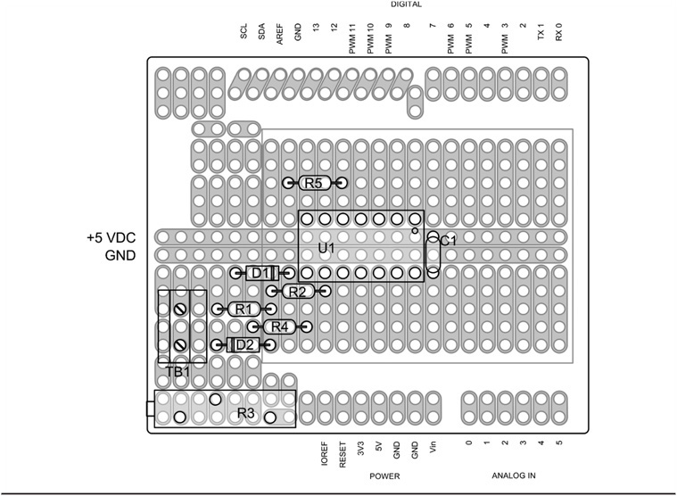
FIGURE 5-4 Parts layout for the general purpose panel meter shield.

We use the same wiring techniques described in the preceding chapters, solid 24 AWG, bare wire with Teflon tubing as insulation where needed. Figure 5-5 shows how we wired up this version of the panel meter. We have left ample room for additional circuitry to be added at a future time.

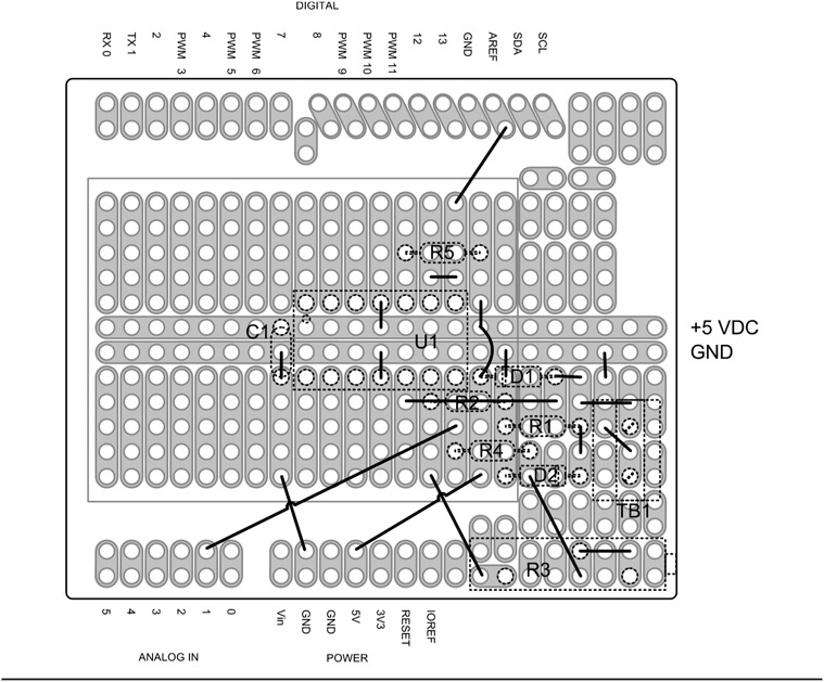
FIGURE 5-5 Wiring diagram for the general purpose panel meter.

The actual wiring on the bottom side of the shield is shown in Figure 5-6. The top side of the shield is shown in Figure 5-7. There is lots of space for additional circuitry in the future. The completed stack of shields and the Arduino board is shown in Figure 5-8. All that remains is to download the software and then test and perform the calibration of the panel meter.

FIGURE 5-6 Bottom view showing wiring of general purpose panel meter shield.

FIGURE 5-7 View of completed general purpose panel meter shield with LCD removed.

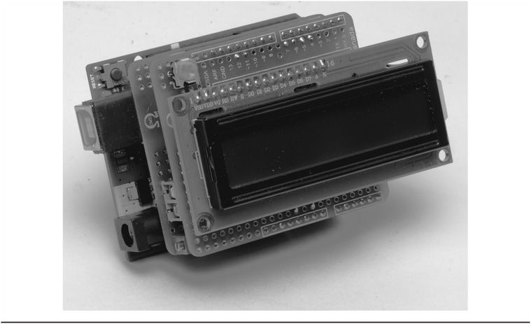
FIGURE 5-8 The completed general purpose panel meter.

An Alternate Design Layout

As an alternative, a panel meter was also constructed on a single Mega shield. Using a Mega shield instead of a simple Arduino shield allows room for the input “conditioning” circuitry and also leaves room for future projects that employ the panel meter. In this alternative version, rather than using the LCD shield constructed in Chapter 3, we chose to mount the LCD display directly to the meter shield using socket headers so that the display may be removed to add other projects. Figure 5-9 shows the top of the shield and component placement. This particular Mega shield has only two buses: one for Vcc (+ 5 VDC) and a second for ground. There are no other interconnected pins that we can use. Connections to the header pins are made in the same manner as shown in Chapter 3, Figures 3-16 through 3-19. The wire is wrapped around the stubby end of the pin and soldered. You can see this on the bottom side of the shield in Figure 5-10.

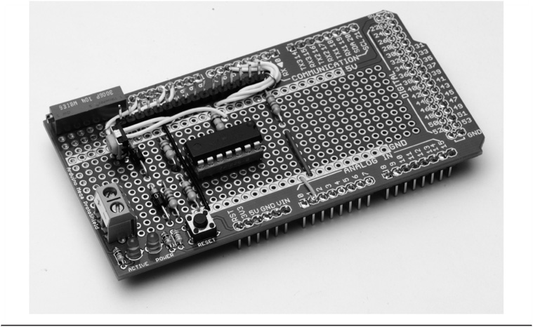
FIGURE 5-9 General purpose panel meter alternative Mega shield layout.

FIGURE 5-10 General purpose panel meter alternative Mega shield layout showing wiring.

The completed alternative design is shown in Figure 5-11 with the LCD installed. Note that the parts and the circuit are the same, only the position of the parts is different and so is the shield when compared to the first version of the meter.

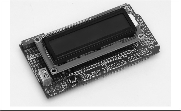
FIGURE 5-11. Completed alternative general purpose panel meter.

 

Loading the Example Software and Testing

The general purpose panel meter software sketch is provided in Listing 5-1. Use the Arduino IDE to compile and upload the sketch into your project.

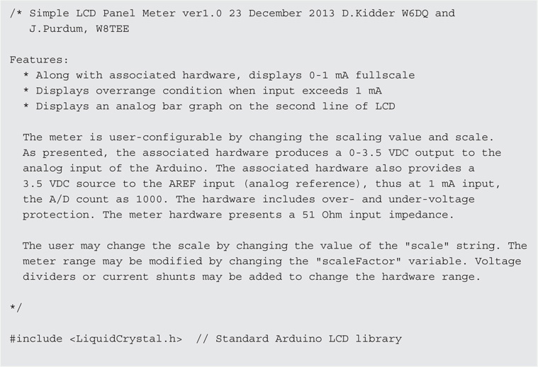
LISTING 5-1 The general purpose panel meter program.

 

WARNING: One very important point while uploading, DO NOT upload the sketch for the first time with the panel meter shield in place. To do so can seriously damage your Arduino. As mentioned earlier, the Arduino is designed to allow an external reference voltage for the A/D converters. The general purpose panel meter shield places a reference voltage on the AREF pin and unfortunately, the internal reference voltage is connected directly to the external reference voltage until the AREF pin is assigned in the code as using an external source. The best practice here is to compile and upload the code, disconnect your USB cable from the Arduino, install the panel meter shield, and then reconnect the USB cable. This prevents you from damaging the Atmel processor.

The software written for the general purpose panel meter uses two libraries. One we have used before with the LCD shield in Chapter 3. The second is a new library that we haven’t used before and is the LCD Bar Graph library and may be freely downloaded from the Arduino “Playground” at:

http://playground.arduino.cc/Code/LcdBarGraph#Download

The latest version of the library as of this writing is 1.4.

Code Walk-Through

There are two libraries used here. The first is one we are familiar with and is the LCD library LiquidCrystal.h that is part of the Arduino IDE. We have added a new library, LcdBarGraph.h, that allows us to have the analog bar graph on the bottom row of the LCD to represent the numeric value displayed on the top row. Follow the steps described in Chapter 4 for RTClib.h to install LcdBarGraph library files.

DEFAULTPRECISION is used to set the number of decimal places that are shown on the LCD. In this case we used 3, which is probably a bit overambitious. If you think about it, a good rule of thumb for a panel meter is that any reading is going to only be readable to half of the smallest scale division. If the typical meter has 50 scale divisions, half of that would be 1/100 of full scale. Depending on how accurate your calibration source is, one might expect that this meter could achieve the same accuracy, so a better choice might be to use “2” for the number of decimal points.

Of course, you have seen the next line before whenever we use the LCD. LCDNUMCOLS sets up the number of columns to display on the LCD. This is the first time we have used an analog input and the line:

#define SENSORPIN A1

assigns our analog input to be analog pin 1 on the Arduino. (We use A1 instead of 1 to denote the analog pin assignment, as that symbolic designation for analog pin 1 is known by the IDE. We think using A1 better documents the fact that analog pin 1 is being used in the assignment statement.) The analog input uses an analog to digital converter, or ADC, to provide a digital representation of the analog value. The ADC is a 10-bit device meaning that the output provides a count of 210 or a range of values between 0000 and 1023 (decimal).

The next two lines are very important for tailoring the meter to your application. These are the scale and scaleFactor definitions. The character string defined by scale allows you to display the units of measurement of your meter. We have used the string mA because our meter is a milliammeter. You can replace this string with anything you would wish to use. Maybe you are measuring speed, so “furlongs per fortnight” might be your desire. Unfortunately, that one won’t fit, as there are only 9 positions on the display for the scale (unless you change the default precision to 2, in which case there would be 10 positions), so you might use “flngs/fort” as your units. You may be just as likely to use “Amperes” or “Volts.”

The scale factor is equally important in that it determines the full-scale value that you can display. The default is a trivial case where 1000 counts on the ADC is equal to a displayed value of 1.000 mA. But what if you wish to display 20 V as the full-scale value? Take a look at the line a little bit farther down in the code within the “loop” portion of the code. The line:

val = (float) analogIn / scaleFactor;

dtostrf(val, VALUEWIDTH, DEFAULTPRECISION, buffer);

is the one we are interested in. Ignoring the function call dtostrf() for the moment, here we read the analog input on analog pin 1 and divide by the scale factor and assign it into val. In this example, we want the count of 1000 to equal 20.00 so the scale factor would be 50 because 1000 divided by 50 would result in a value of 20.00. We discuss scale factor a bit more when we talk about the hardware side of changing the scale and range in an upcoming section.

Instantiating the lcd and lbg Objects

The line:

LiquidCrystal lcd(12, 11, 5, 4, 3, 2);

is also one we’ve seen before and is used to set up the hardware pins used by the LCD. We are creating an object named lcd using the class named “LiquidCrystal.” The object, lcd, uses the object constructor that asks for the pin numbers that we have chosen for the LCD hardware interface. These pin numbers are passed to the constructor as parameters that initialize the object to talk to our LCD hardware.

The next line is new and is associated with the bar graph library. Look at this line:

LcdBarGraph lbg(&lcd, LCDNUMCOLS, BARGRAPHCOL, BARGRAPHROW);

Here we are calling the C++ LcdBarGraph class constructor to create an object named lbg. The constructor initializes certain members of the class to specific values: 1) a reference (i.e., the memory address, or lvalue, as denoted by the “&” operator) to the object lcd (that was just instantiated), 2) define the number of columns used for the bar graph, and 3) places the start of the bar graph in column 0 of row 1. This places the bar graph in the bottom row of the LCD (remember that the rows and columns start with 0).

We learned about void setup() in Chapter 2. The next line:

analogReference(EXTERNAL);

is how we tell the Arduino to use the AREF pin as an external reference voltage. You recall that the voltage applied to AREF when set to EXTERNAL allows us to have a full count on the ADC (1023) when the analog input voltage is equal to the AREF input.

The next series of statements should also be familiar by now. Each of the statements begins with the object name, lcd. Each statement calls the stated function within an lcd object as defined within the LiquidCrystal class. So lcd.begin(), lcd.clear(), lcd.home(), lcd.print(), and lcd.setCursor() are all class methods available to perform some specific action on the display. We use lcd.begin() to set the number of rows and columns that are to be used by the display. We then use lcd.print() to display a “splash screen,” which is a way of telling us that the program is starting. We move the cursor to the next row with lcd.setCursor() and display the version and date of the program. In order to keep the splash screen on the display long enough to read it, we add a little time delay with delay(), in this instance, 3 seconds (3000 milliseconds) and then call lcd.clear() to clear the display. (We avoid using the clear() method outside of the one call in setup() because it is fairly slow.)

The loop() Code

The first dozen lines or so of the loop() function simply establish the working variables and call analogRead() to fetch the current value of the analog input. The value returned in analogIn is then scaled and assigned into val. The dtostrf() function is a standard library function that was added to the Arduino IDE in the post-1.0 era. The dtostrf() function converts a double data type to an ASCII string using a floating point format that is specified by its arguments. The parameter VALUEWIDTH is the total number of characters you want the string to use, including the decimal point and a minus sign (if applicable). Because we only have 16 columns to work with, we arbitrarily set VALUEWIDTH to 6. The symbolic constant DEFAULTPRECISION is the number of digits you want displayed after the decimal point. We set DEFAULTPRECISION to 3. The final argument, buffer[], is where we want to store the result after the conversion. The dtostrf() function returns a pointer to char, so we could nest the function call in a print() (or other) function call if needed.

After the dtostrf() function call, buffer[] contains the ASCII representation of the value read by analogRead(). Because we now want to append the appropriate scale value to the string, we use the following code:

     

If you walk through this code snippet, you should be able to convince yourself that, after the while loop finishes, buffer[] contains a string with the measured analog value and its scale (e.g., “.123 mA”). The code then moves buffer[] to the LCD display. When studying the code, it helps to remember that VALUEWIDTH characters were written to buffer[] during the dtostrf() call and that we added a space character after that number. That hint should help you ferret out what buffer [VALUEWIDTH + 1 + i] is all about.

Earlier we discussed the concept of having an overrange value for the analog input. In other words, we want to provide a means of determining that the input value is greater than our full-scale display value of 1.000 mA. We know what the hardware does, but now we have to provide the software to complete the job. One way to look at the notion of overrange is to say that the analog input value exists in one of two “states.” One state is within range and the other is out of range. We know that the only possible values for the analog input are within the counts of 0000 through 1023. To break this down a bit further, the values that exist “within range” are from the count 0000 through 1000, and the counts that are “out of range” exist from 1001 through 1023. Because there are only two possible states, a simple if statement:

if (analogIn <= MAXANALOGVALUE) {

determines which state currently exits for the analog input value.

If the analog input value can be displayed properly, the current state is such that we can display the bar graph to depict its value. The bar graph uses the lbg object to draw the bar graph using the scaled value, val, to draw the bar graph within the range established by MAXANALOGVALUE. The code then calls delay() to allow the LCD to update the display. (Again, delay() is okay to use provided you don’t have the Arduino doing something important in the background. The reason is because delay() shuts down most of the board’s functionality during the delay period. Interrupt service routines, however, can still be serviced.)

If the analog value causes an out-of-range state to exist, the bar graph is not displayed. The else condition of the if test causes “Overrange!” to be displayed on the second line of the display. The entire display is then blinked by calls to lcd.noDisplay() and lcd.display() with ERRORDELAY pauses between the calls.

 

Testing and Calibration of the Meter

Once you have completed construction of the meter, three steps remain. First, you need to compile and upload the code presented in Listing 5-1. Second, you need to test the meter to make sure it is working properly. Third, after you know the meter is working, you need to calibrate it. It is the second and third steps that we discuss in this section.

To test the meter, you need do nothing more than provide a reliable 1 mA current source. So, how do you do that? A simple way is to use a 9 V transistor radio battery and a resistor. You can employ Ohm’s law (E = I × R) to determine the value of series resistor to produce 1 mA of current. And, oh by the way, in doing so you have created a nice tool to calibrate the meter!

So, 9 V at 1 mA results in a resistor value of 9 kΩ. However, that is a nonstandard value for 5% resistors. One solution is to purchase a precision resistor of 1% or better tolerance. But do you really need to do that? If you know the real value of the resistor and the real voltage of the battery, you can determine the real current. Also, a fresh 9 V transistor radio battery often has a voltage higher than 9 V! A used battery normally is much less than its rated voltage. Hopefully, you have a multimeter that you can use to measure the voltage and the resistor value. If not, Harbor Freight is a good source for an inexpensive digital multimeter! Or, maybe you can borrow one from a friend who does. Other potential sources for a multimeter are another ham, the physics department at your local high school, community college, or university. Most are happy to allow you to bring in your resistor and battery and use their equipment. Once you know the real current, it is a simple matter of adjusting the 10-turn pot to the correct displayed value.

 

Changing the Meter Range and Scale

You now have a digital panel meter that can read current up to 1 mA. But what if you need to measure the output of a solar charger? Or perhaps the current being delivered by the solar panel? You need to “scale” the meter to the desired range you want to measure. To do this, you add “scaling circuits” to the meter. You can also change the “units” displayed on the LCD by a simple change to the software. This section describes how these changes are made.

Few applications require a meter that only reads 0–1 mA. More often the case is that a meter is needed to measure a voltage, say 0–150 VDC, or a higher current, 0–10 A. Well, there is a solution. You can add series resistors to create a voltmeter or a shunt resistor to create an ammeter. Because you know that 50 mV across the input resistor creates a 1 mA full-scale reading, it is a simple matter using Ohm’s law to determine the correct value to use as a scaling resistor. Figure 5-12 shows the basic circuits used for scaling. The dashed lines are the existing circuitry of the panel meter.

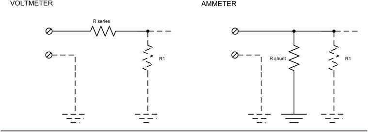
FIGURE 5-12 Scaling circuits.

Voltmeter

In the voltmeter circuit of Figure 5-12, a series resistor is added to form a voltage divider. You know that the voltage across the input of our meter needs to be 50 mV (or 0.05 V) across R1 for a full-scale reading. You also know that two resistors in series carry the same current and we know that the full-scale current is 1 mA. Therefore if you subtract 50 mV from the full-scale reading you want, you can then use Ohm’s law to determine the missing resistor value that must be added into the circuit.

For example, let’s say you want to construct a voltmeter with a full-scale reading of 15 VDC. To determine the value of the series resistor, you subtract 0.05 V from 15 V and then divide the result by 0.001 A (1 mA). Some quick math indicates the resultant value is 14,950 Ω. When we consider all of the accumulated tolerance errors of the resistors in this circuit, a good old 15K Ω resistor should work just fine. Remember that there is a potentiometer in the meter circuit that allows for calibration of the full-scale reading.

One thing that is important to remember for all of these circuits is power dissipation. Any current flowing through a resistor creates heat and the resistor must have a sufficient power rating (P) to handle the heat load generated. P = I × E, or to put it another way, P = I² × R. So, in this case, with 0.001 A and 15K Ω, the power dissipated is 0.015 W. So, a ¼ W resistor is more than adequate for this application.

Ammeter

In the ammeter circuit, a shunt resistor is added to “divert” some of the current from the meter. In this case, the important thing to remember is that two resistors in parallel have the same voltage across the two of them, and that the total current is the sum of the current through each resistor. R1 is the meter input resistor and, by design, draws 1 mA at 50 mV. This means you can subtract 1 mA from the total current you wish to measure. Divide 50 mV by that result and you have the value of the required shunt resistor.

For example, let’s say we need to measure up to 500 mA DC current. Our total current to be measured is 500 mA and we can then subtract the current through the meter to determine the current through the shunt. So, 500 – 1 = 499 mA or 0.499 A. Divide this by the voltage, 0.05 (50 mV), and we get 0.1002 Ω. The power rating of this resistor would be 0.499 A times 0.05 V or 0.025 W.

Let’s take this example into the real world. How do you find a 0.1 Ω resistor with a 0.025 W rating? Well, you don’t. But, we can make one using other resistors. Ten 1 Ω resistors in parallel make a dandy 0.1 Ω resistor. And if you use ¼ W or even ⅛ W resistors, there is more than enough power dissipation to meet our requirements. Remember that these resistors are not exactly what they say they are. There is a tolerance rating for them. Tolerance rating means that, at a specified resistance, the actual resistance value is somewhere within that tolerance range. If we use 5% tolerance resistors, it means that the final value of a 1 Ω resistor is somewhere between 0.095 and 1.05 Ω. Again, you use the 10-turn pot on the meter shield to adjust your meter for the proper full-scale reading.

Changing the Scale

Obviously, if you change the way the meter scales the readings, you also need to change the scale of the meter. Changing the scale is quite simple. It is merely a matter of editing the character string variable char scale[] to the desired value. As coded, the current scale is in milliamps; “mA” in Listing 5-1. Use the Arduino IDE to replace “mA” with the desired character sequence, say, “Volts,” or “Amperes,” as the case may be.

 

Conclusion

There are many things that can be “tweaked” in this design. For instance, maybe you want the basic meter to read a different full-scale value other than 1 mA. Well, it is a matter of adjusting the gain of the op amp circuit and possibly changing the scale factor in the code. Such modifications are left as a (kinda fun) exercise for the reader. For the more ambitious hardware types, one possible change is to provide a true differential input that doesn’t require a ground reference. If you want to explore the software, maybe adding meter “ballistics.” That is, account for the fact that an analog meter pointer has some mass to it and exhibits accelerations and time lags. Another possibility is to add a peak reading indicator. One might explore how to add those features to this project. You could also add a switch that would toggle different resistor combinations for different meter ranges, with software modifications to change the scale automatically.

This project provides a simple to construct and simple to use general purpose panel meter. How it can be used is really up to your imagination.