
Chapter 1. Audio Principles
1.1. The Physics of Sound
Sound is simply an airborne version of vibration. The air which carries sound is a mixture of gases. In gases, the molecules contain so much energy that they break free from their neighbors and rush around at high speed. As Figure 1.1(a) shows, the innumerable elastic collisions of these high-speed molecules produce pressure on the walls of any gas container. If left undisturbed in a container at a constant temperature, eventually the pressure throughout would be constant and uniform.
Figure 1.1. (a) The pressure exerted by a gas is due to countless elastic collisions between gas molecules and the walls of the container. (b) If the wall moves against the gas pressure, the rebound velocity increases. (c) Motion with the gas pressure reduces the particle velocity.


Sound disturbs this simple picture. Figure 1.1(b) shows that a solid object which moves against gas pressure increases the velocity of the rebounding molecules, whereas in Figure 1.1(c) one moving with gas pressure reduces that velocity. The average velocity and the displacement of all the molecules in a layer of air near a moving body is the same as the velocity and displacement of the body. Movement of the body results in a local increase or decrease in pressure of some kind. Thus sound is both a pressure and a velocity disturbance.
Despite the fact that a gas contains endlessly colliding molecules, a small mass or particle of gas can have stable characteristics because the molecules leaving are replaced by new ones with identical statistics. As a result, acoustics seldom need to consider the molecular structure of air and the constant motion can be neglected. Thus when particle velocity and displacement are considered, this refers to the average values of a large number of molecules. In an undisturbed container of gas, the particle velocity and displacement will both be zero everywhere.
When the volume of a fixed mass of gas is reduced, the pressure rises. The gas acts like a spring; it is compliant. However, a gas also has mass. Sound travels through air by an interaction between the mass and the compliance. Imagine pushing a mass via a spring. It would not move immediately because the spring would have to be compressed in order to transmit a force. If a second mass is connected to the first by another spring, it would start to move even later. Thus the speed of a disturbance in a mass/spring system depends on the mass and the stiffness. Sound travels through air without a net movement of the air.
The speed of sound is proportional to the square root of the absolute temperature. On earth, temperature changes with respect to absolute zero (−273°C) also amount to around 1% except in extremely inhospitable places. The speed of sound experienced by most of us is about 1000 ft per second or 344 m per second.
1.2. Wavelength
Sound can be due to a one-off event known as percussion, or a periodic event such as the sinusoidal vibration of a tuning fork. The sound due to percussion is called transient, whereas a periodic stimulus produces steady-state sound having a frequency f.
Because sound travels at a finite speed, the fixed observer at some distance from the source will experience the disturbance at some later time. In the case of a transient sound caused by an impact, the observer will detect a single replica of the original as it passes at the speed of sound. In the case of the tuning fork, a periodic sound source, the pressure peaks and dips follow one another away from the source at the speed of sound. For a given rate of vibration of the source, a given peak will have propagated a constant distance before the next peak occurs. This distance is called the wavelength lambda. Figure 1.2 shows that wavelength is defined as the distance between any two identical points on the whole cycle. If the source vibrates faster, successive peaks get closer together and the wavelength gets shorter. Figure 1.2 also shows that the wavelength is inversely proportional to the frequency. It is easy to remember that the wavelength of 1000 Hz is a foot (about 30 cm).
Figure 1.2. Wavelength is defined as the distance between two points at the same place on adjacent cycles. Wavelength is inversely proportional to frequency.

1.3. Periodic and Aperiodic Signals
Sounds can be divided into these two categories and analyzed either in the time domain in which the waveform is considered or in the frequency domain in which the spectrum is considered. The time and frequency domains are linked by transforms of which the best known is the Fourier transform.
Figure 1.3(a) shows that an ideal periodic signal is one which repeats after some constant time has elapsed and goes on indefinitely in the time domain. In the frequency domain such a signal will be described as having a fundamental frequency and a series of harmonics or partials that are at integer multiples of the fundamental. The timbre of an instrument is determined by the harmonic structure. Where there are no harmonics at all, the simplest possible signal results that has only a single frequency in the spectrum. In the time domain this will be an endless sine wave.
Figure 1.3. (a) A periodic signal repeats after a fixed time and has a simple spectrum consisting of fundamental plus harmonics. (b) An aperiodic signal such as noise does not repeat and has a continuous spectrum. (c) A transient contains an anharmonic spectrum.


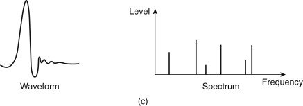
Figure 1.3(b) shows an aperiodic signal known as white noise. The spectrum shows that there is an equal level at all frequencies, hence the term “white,” which is analogous to the white light containing all wavelengths. Transients or impulses may also be aperiodic. A spectral analysis of a transient [Figure 1.3(c)] will contain a range of frequencies, but these are not harmonics because they are not integer multiples of the lowest frequency. Generally the narrower an event in the time domain, the broader it will be in the frequency domain and vice versa.
1.4. Sound and the Ear
Experiments can tell us that the ear only responds to a certain range of frequencies within a certain range of levels. If sound is defined to fall within those ranges, then its reproduction is easier because it is only necessary to reproduce those levels and frequencies that the ear can detect.
Psychoacoustics can describe how our hearing has finite resolution in both time and frequency domains such that what we perceive is an inexact impression. Some aspects of the original disturbance are inaudible to us and are said to be masked. If our goal is the highest quality, we can design our imperfect equipment so that the shortcomings are masked. Conversely, if our goal is economy we can use compression and hope that masking will disguise the inaccuracies it causes.
A study of the finite resolution of the ear shows how some combinations of tones sound pleasurable whereas others are irritating. Music has evolved empirically to emphasize primarily the former. Nevertheless, we are still struggling to explain why we enjoy music and why certain sounds can make us happy whereas others can reduce us to tears. These characteristics must still be present in digitally reproduced sound.
The frequency range of human hearing is extremely wide, covering some 10 octaves (an octave is a doubling of pitch or frequency) without interruption.
By definition, the sound quality of an audio system can only be assessed by human hearing. Many items of audio equipment can only be designed well with a good knowledge of the human hearing mechanism. The acuity of the human ear is finite but astonishing. It can detect tiny amounts of distortion and will accept an enormous dynamic range over a wide number of octaves. If the ear detects a different degree of impairment between two audio systems in properly conducted tests, we can say that one of them is superior.
However, any characteristic of a signal that can be heard can, in principle, also be measured by a suitable instrument, although in general the availability of such instruments lags the requirement. The subjective tests will tell us how sensitive the instrument should be. Then the objective readings from the instrument give an indication of how acceptable a signal is in respect of that characteristic.
The sense we call hearing results from acoustic, mechanical, hydraulic, nervous, and mental processes in the ear/brain combination, leading to the term psychoacoustics. It is only possible to briefly introduce the subject here. The interested reader is referred to Moore[1] for an excellent treatment.
Figure 1.4 shows that the structure of the ear is divided into outer, middle, and inner ears. The outer ear works at low impedance, the inner ear works at high impedance, and the middle ear is an impedance matching device. The visible part of the outer ear is called the pinna, which plays a subtle role in determining the direction of arrival of sound at high frequencies. It is too small to have any effect at low frequencies. Incident sound enters the auditory canal or meatus. The pipe-like meatus causes a small resonance at around 4 kHz. Sound vibrates the eardrum or tympanic membrane, which seals the outer ear from the middle ear. The inner ear or cochlea works by sound traveling though a fluid. Sound enters the cochlea via a membrane called the oval window.
Figure 1.4. The structure of the human ear. See text for details.

If airborne sound were to be incident on the oval window directly, the serious impedance mismatch would cause most of the sound to be reflected. The middle ear remedies that mismatch by providing a mechanical advantage. The tympanic membrane is linked to the oval window by three bones known as ossicles, which act as a lever system such that a large displacement of the tympanic membrane results in a smaller displacement of the oval window but with greater force. Figure 1.5 shows that the malleus applies a tension to the tympanic membrane, rendering it conical in shape. The malleus and the incus are firmly joined together to form a lever. The incus acts on the stapes through a spherical joint. As the area of the tympanic membrane is greater than that of the oval window, there is further multiplication of the available force. Consequently, small pressures over the large area of the tympanic membrane are converted to high pressures over the small area of the oval window.
Figure 1.5. The malleus tensions the tympanic membrane into a conical shape. The ossicles provide an impedance-transforming lever system between the tympanic membrane and the oval window.

The middle ear is normally sealed, but ambient pressure changes will cause static pressure on the tympanic membrane, which is painful. The pressure is relieved by the Eustachian tube, which opens involuntarily while swallowing. The Eustachian tubes open into the cavities of the head and must normally be closed to avoid one’s own speech appearing deafeningly loud.
The ossicles are located by minute muscles, which are normally relaxed. However, the middle ear reflex is an involuntary tightening of the tensor tympani and stapedius muscles, which heavily damp the ability of the tympanic membrane and the stapes to transmit sound by about 12 dB at frequencies below 1 kHz. The main function of this reflex is to reduce the audibility of one’s own speech. However, loud sounds will also trigger this reflex, which takes some 60 to 120 ms to occur, too late to protect against transients such as gunfire.
1.5. The Cochlea
The cochlea, shown in Figure 1.6(a), is a tapering spiral cavity within bony walls, which is filled with fluid. The widest part, near the oval window, is called the base and the distant end is the apex. Figure 1.6(b) shows that the cochlea is divided lengthwise into three volumes by Reissner’s membrane and the basilar membrane. The scala vestibuli and the scala tympani are connected by a small aperture at the apex of the cochlea known as the helicotrema. Vibrations from the stapes are transferred to the oval window and become fluid pressure variations, which are relieved by the flexing of the round window. Essentially the basilar membrane is in series with the fluid motion and is driven by it except at very low frequencies where the fluid flows through the helicotrema, bypassing the basilar membrane.
Figure 1.6. (a) The cochlea is a tapering spiral cavity. (b) The cross section of the cavity is divided by Reissner’s membrane and the basilar membrane. (c) The basilar membrane tapers so that its resonant frequency changes along its length.

The vibration of the basilar membrane is sensed by the organ of Corti, which runs along the center of the cochlea. The organ of Corti is active in that it contains elements that can generate vibration as well as sense it. These are connected in a regenerative fashion so that the Q factor, or frequency selectivity of the ear, is higher than it would otherwise be. The deflection of hair cells in the organ of Corti triggers nerve firings and these signals are conducted to the brain by the auditory nerve. Some of these signals reflect the time domain, particularly during the transients with which most real sounds begin and also at low frequencies. During continuous sounds, the basilar membrane is also capable of performing frequency analysis.
Figure 1.6(c) shows that the basilar membrane is not uniform, but tapers in width and varies in thickness in the opposite sense to the taper of the cochlea. The part of the basilar membrane that resonates as a result of an applied sound is a function of the frequency. High frequencies cause resonance near the oval window, whereas low frequencies cause resonances further away. More precisely, the distance from the apex where the maximum resonance occurs is a logarithmic function of the frequency. Consequently, tones spaced apart in octave steps will excite evenly spaced resonances in the basilar membrane. The prediction of resonance at a particular location on the membrane is called place theory. Essentially the basilar membrane is a mechanical frequency analyzer.
Nerve firings are not a perfect analog of the basilar membrane motion. On continuous tones, a nerve firing appears to occur at a constant phase relationship to the basilar vibration, a phenomenon called phase locking, but firings do not necessarily occur on every cycle. At higher frequencies firings are intermittent, yet each is in the same phase relationship.
The resonant behavior of the basilar membrane is not observed at the lowest audible frequencies below 50 Hz. The pattern of vibration does not appear to change with frequency and it is possible that the frequency is low enough to be measured directly from the rate of nerve firings.
1.6. Mental Processes
The nerve impulses are processed in specific areas of the brain that appear to have evolved at different times to provide different types of information. The time domain response works quickly, primarily aiding the direction-sensing mechanism and is older in evolutionary terms. The frequency domain response works more slowly, aiding the determination of pitch and timbre and evolved later, presumably as speech evolved.
The earliest use of hearing was as a survival mechanism to augment vision. The most important aspect of the hearing mechanism was the ability to determine the location of the sound source. Figure 1.7 shows that the brain can examine several possible differences between the signals reaching the two ears. In Figure 1.7(a), a phase shift is apparent. In Figure 1.7(b), the distant ear is shaded by the head, resulting in a different frequency response compared to the nearer ear. In Figure 1.7(c), a transient sound arrives later at the more distant ear. The interaural phase, delay, and level mechanisms vary in their effectiveness depending on the nature of the sound to be located. At some point a fuzzy logic decision has to be made as to how the information from these different mechanisms will be weighted.
Figure 1.7. Having two spaced ears is cool. (a) Off-center sounds result in a phase difference. (b) The distant ear is shaded by the head, producing a loss of high frequencies. (c) The distant ear detects transient later.

There will be considerable variation with frequency in the phase shift between the ears. At a low frequency such as 30 Hz, the wavelength is around 11.5 m so this mechanism must be quite weak at low frequencies. At high frequencies the ear spacing is many wavelengths, producing a confusing and complex phase relationship. This suggests a frequency limit of around 1500 Hz, which has been confirmed experimently.
At low and middle frequencies, sound will diffract round the head sufficiently well that there will be no significant difference between the levels at the two ears. Only at high frequencies does sound become directional enough for the head to shade the distant ear, causing what is called interaural intensity difference.
Phase differences are only useful at low frequencies and shading only works at high frequencies. Fortunately, real-world noises and sounds are broadband and often contain transients. Timbral, broadband, and transient sounds differ from tones in that they contain many different frequencies. Pure tones are rare in nature.
A transient has a unique aperiodic waveform, which, as Figure 1.7(c) shows, suffers no ambiguity in the assessment of interaural delay (IAD) between two versions. Note that a one-degree change in sound location causes an IAD of around 10 μs. The smallest detectable IAD is a remarkable 6 μs. This should be the criterion for spatial reproduction accuracy.
Transient noises produce a one-off pressure step whose source is accurately and instinctively located. Figure 1.8 shows an idealized transient pressure waveform following an acoustic event. Only the initial transient pressure change is required for location. The time of arrival of the transient at the two ears will be different and will locate the source laterally within a processing delay of around a millisecond.
Figure 1.8. A real acoustic event produces a pressure step. The initial step is used for spatial location; equalization time signifies the size of the source. (Courtesy of Manger Schallwandlerbau.)

Following the event that generated the transient, the air pressure equalizes. The time taken for this equalization varies and allows the listener to establish the likely size of the sound source. The larger the source, the longer the pressure–equalization time. Only after this does the frequency analysis mechanism tell anything about the pitch and timbre of the sound.
The aforementioned results suggest that anything in a sound reproduction system that impairs the reproduction of a transient pressure change will damage localization and the assessment of the pressure–equalization time. Clearly, in an audio system that claims to offer any degree of precision, every component must be able to reproduce transients accurately and must have at least a minimum phase characteristic if it cannot be phase linear. In this respect, digital audio represents a distinct technical performance advantage, although much of this is later lost in poor transducer design, especially in loudspeakers.
1.7. Level and Loudness
At its best, the ear can detect a sound pressure variation of only 2×10⁻⁵ Pascals root mean square (rms) and so this figure is used as the reference against which the sound pressure level (SPL) is measured. The sensation of loudness is a logarithmic function of SPL; consequently, a logarithmic unit, the decibel, was adopted for audio measurement. The decibel is explained in detail in Section 1.12.
The dynamic range of the ear exceeds 130 dB, but at the extremes of this range, the ear either is straining to hear or is in pain. The frequency response of the ear is not at all uniform and it also changes with SPL. The subjective response to level is called loudness and is measured in phons. The phon scale is defined to coincide with the SPL scale at 1 kHz, but at other frequencies the phon scale deviates because it displays the actual SPLs judged by a human subject to be equally loud as a given level at 1 kHz. Figure 1.9 shows the so-called equal loudness contours, which were originally measured by Fletcher and Munson and subsequently by Robinson and Dadson. Note the irregularities caused by resonances in the meatus at about 4 and 13 kHz.
Figure 1.9. Contours of equal loudness showing that the frequency response of the ear is highly level dependent (solid line, age 20; dashed line, age 60).

Usually, people’s ears are at their most sensitive between about 2 and 5 kHz; although some people can detect 20 kHz at high level, there is much evidence to suggest that most listeners cannot tell if the upper frequency limit of sound is 20 or 16 kHz.[2,3] For a long time it was thought that frequencies below about 40 Hz were unimportant, but it is now clear that the reproduction of frequencies down to 20 Hz improves reality and ambience.[4] The generally accepted frequency range for high-quality audio is 20 to 20,000 Hz, although an upper limit of 15,000 Hz is often applied for broadcasting.
The most dramatic effect of the curves of Figure 1.9 is that the bass content of reproduced sound is reduced disproportionately as the level is turned down. This would suggest that if a sufficiently powerful yet high-quality reproduction system is available, the correct tonal balance when playing a good recording can be obtained simply by setting the volume control to the correct level. This is indeed the case. A further consideration is that many musical instruments, as well as the human voice, change timbre with the level and there is only one level that sounds correct for the timbre.
Audio systems with a more modest specification would have to resort to the use of tone controls to achieve a better tonal balance at lower SPL. A loudness control is one where the tone controls are automatically invoked as the volume is reduced. Although well meant, loudness controls seldom compensate accurately because they must know the original level at which the material was meant to be reproduced as well as the actual level in use.
A further consequence of level-dependent hearing response is that recordings that are mixed at an excessively high level will appear bass light when played back at a normal level. Such recordings are more a product of self-indulgence than professionalism.
Loudness is a subjective reaction and is almost impossible to measure. In addition to the level-dependent frequency response problem, the listener uses the sound not for its own sake but to draw some conclusion about the source. For example, most people hearing a distant motorcycle will describe it as being loud. Clearly, at the source, it is loud, but the listener has compensated for the distance.
The best that can be done is to make some compensation for the level-dependent response using weighting curves. Ideally, there should be many, but in practice the A, B, and C weightings were chosen where the A curve is based on the 40-phon response. The measured level after such a filter is in units of dBA. The A curve is almost always used because it most nearly relates to the annoyance factor of distant noise sources.
1.8. Frequency Discrimination
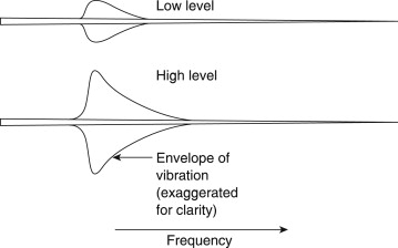
Figure 1.10 shows an uncoiled basilar membrane with the apex on the left so that the usual logarithmic frequency scale can be applied. The envelope of displacement of the basilar membrane is shown for a single frequency at Figure 1.10(a). The vibration of the membrane in sympathy with a single frequency cannot be localized to an infinitely small area, and nearby areas are forced to vibrate at the same frequency with an amplitude that decreases with distance. Note that the envelope is asymmetrical because the membrane is tapering and because of frequency-dependent losses in the propagation of vibrational energy down the cochlea. If the frequency is changed, as in Figure 1.10(b), the position of maximum displacement will also change. As the basilar membrane is continuous, the position of maximum displacement is infinitely variable, allowing extremely good pitch discrimination of about one-twelfth of a semitone, which is determined by the spacing of hair cells.
Figure 1.10. The basilar membrane symbolically uncoiled. (a) Single frequency causes the vibration envelope shown. (b) Changing the frequency moves the peak of the envelope.

In the presence of a complex spectrum, the finite width of the vibration envelope means that the ear fails to register energy in some bands when there is more energy in a nearby band. Within those areas, other frequencies are mechanically excluded because their amplitude is insufficient to dominate the local vibration of the membrane. Thus the Q factor of the membrane is responsible for the degree of auditory masking, defined as the decreased audibility of one sound in the presence of another. Masking is important because audio compression relies heavily on it.
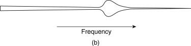
The term used in psychoacoustics to describe the finite width of the vibration envelope is critical bandwidth. Critical bands were first described by Fletcher.[5] The envelope of basilar vibration is a complicated function. It is clear from the mechanism that the area of the membrane involved will increase as the sound level rises. Figure 1.11 shows the bandwidth as a function of level.
Figure 1.11. The critical bandwidth changes with SPL.
As seen elsewhere, transform theory teaches that the higher the frequency resolution of a transform, the worse the time accuracy. As the basilar membrane has finite frequency resolution measured in the width of a critical band, it follows that it must have finite time resolution. This also follows from the fact that the membrane is resonant, taking time to start and stop vibrating in response to a stimulus. There are many examples of this. Figure 1.12 shows the impulse response. Figure 1.13 shows that the perceived loudness of a tone burst increases with duration up to about 200 ms due to the finite response time.
Figure 1.12. Impulse response of the ear showing slow attack and decay as a consequence of resonant behavior.

Figure 1.13. Perceived level of tone burst rises with duration as resonance builds up.

The ear has evolved to offer intelligibility in reverberant environments, which it does by averaging all received energy over a period of about 30 ms. Reflected sound that arrives within this time is integrated to produce a louder sensation, whereas reflected sound that arrives after that time can be temporally discriminated and perceived as an echo. Microphones have no such ability, which is why acoustic treatment is often needed in areas where microphones are used.
A further example of the finite time discrimination of the ear is the fact that short interruptions to a continuous tone are difficult to detect. Finite time resolution means that masking can take place even when the masking tone begins after and ceases before the masked sound. This is referred to as forward and backward masking.[6]
Figure 1.14(a) shows an electrical signal in which two equal sine waves of nearly the same frequency have been added together linearly. Note that the envelope of the signal varies as the two waves move in and out of phase. Clearly the frequency transform calculated to infinite accuracy is that shown at Figure 1.14(b). The two amplitudes are constant and there is no evidence of envelope modulation. However, such a measurement requires an infinite time. When a shorter time is available, the frequency discrimination of the transform falls and the bands in which energy is detected become broader.
Figure 1.14. (a) Result of adding two sine waves of similar frequency. (b) Spectrum of (a) to infinite accuracy. (c) With finite accuracy, only a single frequency is distinguished whose amplitude changes with the envelope of (a) giving rise to beats.


When the frequency discrimination is too wide to distinguish the two tones as shown in Figure 1.14(c), the result is that they are registered as a single tone. The amplitude of the single tone will change from one measurement to the next because the envelope is being measured. The rate at which the envelope amplitude changes is called beat frequency, which is not actually present in the input signal. Beats are an artifact of finite frequency resolution transforms. The fact that human hearing produces beats from pairs of tones proves that it has finite resolution.
1.9. Frequency Response and Linearity
It is a goal in high-quality sound reproduction that the timbre of the original sound shall not be changed by the reproduction process. There are two ways in which timbre can inadvertently be changed, as Figure 1.15 shows. In Figure 1.15(a), the spectrum of the original shows a particular relationship between harmonics. This signal is passed through a system [Figure 1.15 (b)] that has an unequal response at different frequencies. The result is that the harmonic structure [Figure 1.15(c)] has changed, and with it the timbre. Clearly a fundamental requirement for quality sound reproduction is that the response to all frequencies should be equal.
Figure 1.15. Why frequency response matters. (a) Original spectrum determines the timbre of sound. If the original signal is passed through a system with a deficient frequency response (b), the timbre will be changed (c).


Frequency response is easily tested using sine waves of constant amplitude at various frequencies as an input and noting the output level for each frequency.
Figure 1.16 shows that another way in which timbre can be changed is by nonlinearity. All audio equipment has a transfer function between the input and the output, which form the two axes of a graph. Unless the transfer function is exactly straight or linear, the output waveform will differ from the input. A nonlinear transfer function will cause distortion, which changes the distribution of harmonics and changes timbre.
Figure 1.16. Nonlinearity of the transfer function creates harmonies by distorting the waveform. Linearity is extremely important in audio equipment.

At a real microphone placed before an orchestra a multiplicity of sounds may arrive simultaneously. Because the microphone diaphragm can only be in one place at a time, the output waveform must be the sum of all the sounds. An ideal microphone connected by ideal amplification to an ideal loudspeaker will reproduce all of the sounds simultaneously by linear superimposition. However, should there be a lack of linearity anywhere in the system, the sounds will no longer have an independent existence, but will interfere with one another, changing one another’s timbre and even creating new sounds that did not previously exist. This is known as intermodulation. Figure 1.17 shows that a linear system will pass two sine waves without interference. If there is any nonlinearity, the two sine waves will intermodulate to produce sum and difference frequencies, which are easily observed in the otherwise pure spectrum.
Figure 1.17. (a) A perfectly linear system will pass a number of superimposed waveforms without interference so that the output spectrum does not change. (b) A nonlinear system causes intermodulation where the output spectrum contains sum and difference frequencies in addition to the originals.


1.10. The Sine Wave
As the sine wave is such a useful concept it will be treated here in detail. Figure 1.18 shows a constant speed rotation viewed along the axis so that the motion is circular. Imagine, however, the view from one side in the plane of the rotation. From a distance, only a vertical oscillation will be observed and if the position is plotted against time the resultant waveform will be a sine wave. Geometrically, it is possible to calculate the height or displacement because it is the radius multiplied by the sine of the phase angle.
Figure 1.18. A sine wave is one component of a rotation. When a rotation is viewed from two places at places at right angles, one will see a sine wave and the other will see a cosine wave. The constant phase shift between sine and cosine is 90° and should not be confused with the time variant phase angle due to the rotation.

The phase angle is obtained by multiplying the angular velocity ω by the time t. Note that the angular velocity is measured in radians per second, whereas frequency f is measured in rotations per second or hertz. As a radian is unit distance at unit radius (about 57°), then there are 2π radians in one rotation. Thus the phase angle at a time t is given by sinωt or sin2πft.
A second viewer, who is at right angles to the first viewer, will observe the same waveform but with different timing. The displacement will be given by the radius multiplied by the cosine of the phase angle. When plotted on the same graph, the two waveforms are phase shifted with respect to one another. In this case the phase shift is 90° and the two waveforms are said to be in quadrature. Incidentally, the motions on each side of a steam locomotive are in quadrature so that it can always get started (the term used is quartering). Note that the phase angle of a signal is constantly changing with time, whereas the phase shift between two signals can be constant. It is important that these two are not confused.
The velocity of a moving component is often more important in audio than the displacement. The vertical component of velocity is obtained by differentiating the displacement. As the displacement is a sine wave, the velocity will be a cosine wave whose amplitude is proportional to frequency. In other words, the displacement and velocity are in quadrature with the velocity lagging. This is consistent with the velocity reaching a minimum as the displacement reaches a maximum and vice versa. Figure 1.19 shows displacement, velocity, and acceleration waveforms of a body executing simple harmonic motion (SHM). Note that the acceleration and the displacement are always antiphase.
Figure 1.19. The displacement, velocity, and acceleration of a body executing simple harmonic motion (SHM).

1.11. Root Mean Square Measurements
Figure 1.20(a) shows that, according to Ohm’s law, the power dissipated in a resistance is proportional to the square of the applied voltage. This causes no difficulty with direct current (DC), but with alternating signals such as audio it is harder to calculate the power. Consequently, a unit of voltage for alternating signals was devised. Figure 1.20(b) shows that the average power delivered during a cycle must be proportional to the mean of the square of the applied voltage. Since power is proportional to the square of applied voltage, the same power would be dissipated by a DC voltage whose value was equal to the square root of the mean of the square of the AC voltage. Thus the volt rms was specified. An AC signal of a given number of volts rms will dissipate exactly the same amount of power in a given resistor as the same number of volts DC.
Figure 1.20. (a) Ohm’s law: the power developed in a resistor is proportional to the square of the voltage. Consequently, 1 mW in 600 Ω requires 0.775 V. With a sinusoidal alternating input (b), the power is a sine-squared function, which can be averaged over one cycle. A DC voltage that delivers the same power has a value that is the square root of the mean of the square of the sinusoidal input to be measured and the reference. The Bel is too large so the decibel (dB) is used in practice. (b) As the dB is defined as a power ratio, voltage ratios have to be squared. This is conveniently done by doubling the logs so that the ratio is now multiplied by 20.


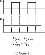
Figure 1.21(a) shows that for a sine wave the rms voltage is obtained by dividing the peak voltage Vpk by the square root of 2. However, for a square wave [Figure 1.21(b)] the rms voltage and the peak voltage are the same. Most moving coil AC voltmeters only read correctly on sine waves, whereas many electronic meters incorporate a true rms calculation.
Figure 1.21. (a) For a sine wave the conversion factor from peak to rms is
![]() . (b) For a square wave the peak and rms voltage are the same.
. (b) For a square wave the peak and rms voltage are the same.

On an oscilloscope it is often easier to measure the peak-to-peak voltage, which is twice the peak voltage. The rms voltage cannot be measured directly on an oscilloscope since it depends on the waveform, although the calculation is simple in the case of a sine wave.
1.12. The Decibel
The first audio signals to be transmitted were on telephone lines. Where the wiring is long compared to the electrical wavelength (not to be confused with the acoustic wavelength) of the signal, a transmission line exists in which the distributed series inductance and the parallel capacitance interact to give the line a characteristic impedance. In telephones this turned out to be about 600 Ω. In transmission lines the best power delivery occurs when the source and the load impedance are the same; this is the process of matching.
It was often required to measure the power in a telephone system, and 1 mW was chosen as a suitable unit. Thus the reference against which signals could be compared was the dissipation of 1 mW in 600 Ω. Figure 1.20(a) shows that the dissipation of 1 mW in 600 Ω will be due to an applied voltage of 0.775 V rms. This voltage became the reference against which all audio levels are compared.
The decibel is a logarithmic measuring system and has its origins in telephony[7] where the loss in a cable is a logarithmic function of the length. Human hearing also has a logarithmic response with respect to sound pressure level. In order to relate to the subjective response, audio signal level measurements also have to be logarithmic and so the decibel was adopted for audio.
Figure 1.22 shows the principle of the logarithm. To give an example, if it is clear that 102 is 100 and 103 is 1000, then there must be a power between 2 and 3 to which 10 can be raised to give any value between 100 and 1000. That power is the logarithm to base 10 of the value, for example, log10 300=2.5 approximately. Note that 100 is 1.
Figure 1.22. (a) The logarithm of a number is the power to which the base (in this case 10) must be raised to obtain the number. (b) Multiplication is obtained by adding logs, division by subtracting. (c) The slide rule has two logarithmic scales whose length can be added or subtracted easily.

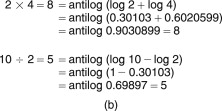

Logarithms were developed by mathematicians before the availability of calculators or computers to ease calculations such as multiplication, squaring, division, and extracting roots. The advantage is that, armed with a set of log tables, multiplication can be performed by adding and division by subtracting. Figure 1.22 shows some examples. It will be clear that squaring a number is performed by adding two identical logs and the same result will be obtained by multiplying the log by 2.
The slide rule is an early calculator, which consists of two logarithmically engraved scales in which the length along the scale is proportional to the log of the engraved number. By sliding the moving scale, two lengths can be added or subtracted easily and, as a result, multiplication and division are readily obtained.
The logarithmic unit of measurement in telephones was called the Bel after Alexander Graham Bell, the inventor. Figure 1.23(a) shows that the Bel was defined as the log of the power ratio between the power to be measured and some reference power. Clearly the reference power must have a level of 0 Bels, as log10 1 is 0.
Figure 1.23. (a) The Bel is the log of the ratio between two powers, that between two powers, that to be measured, and the reference. The Bel is too large so the decibel is used in practice. (b) As the decibel is defined as a power ratio, voltage ratios have to be squared. This is done conveniently by doubling the logs so that the ratio is now multiplied by 20.

The Bel was found to be an excessively large unit for practical purposes and so it was divided into 10 decibels, abbreviated dB with a small d and a large B and pronounced deebee. Consequently, the number of dBs is 10 times the log of the power ratio. A device such as an amplifier can have a fixed power gain that is independent of signal level and this can be measured in dBs. However, when measuring the power of a signal, it must be appreciated that the dB is a ratio and to quote the number of dBs without stating the reference is about as senseless as describing the height of a mountain as 2000 without specifying whether this is feet or meters. To show that the reference is 1 mW into 600 Ω the units will be dB(m). In radio engineering, the dB(W) will be found, which is power relative to 1 W.
Although the dB(m) is defined as a power ratio, level measurements in audio are often done by measuring the signal voltage using 0.775 V as a reference in a circuit whose impedance is not necessarily 600 Ω. Figure 1.23(b) shows that as the power is proportional to the square of the voltage, the power ratio will be obtained by squaring the voltage ratio. As squaring in logs is performed by doubling, the squared term of the voltages can be replaced by multiplying the log by a factor of two. To give a result in dBs, the log of the voltage ratio now has to be multiplied by 20.
While 600 Ω matched impedance working is essential for the long distances encountered with telephones, it is quite inappropriate for analog audio wiring in a studio. The wavelength of audio in wires at 20 kHz is 15 km. Studios are built on a smaller scale than this and clearly analog audio cables are not transmission lines and their characteristic impedance is not relevant.
In professional analog audio systems, impedance matching is not only unnecessary but also undesirable. Figure 1.24(a) shows that when impedance matching is required, the output impedance of a signal source must be raised artificially so that a potential divider is formed with the load. The actual drive voltage must be twice that needed on the cable as the potential divider effect wastes 6 dB of signal level and requires unnecessarily high power supply rail voltages in equipment. A further problem is that cable capacitance can cause an undesirable HF roll-off in conjunction with the high source impedance.
Figure 1.24. (a) Traditional impedance matched source wastes half the signal voltage in the potential divider due to the source impedance and the cable. (b) Modern practice is to use low-output impedance sources with high-impedance loads.


In modern professional analog audio equipment, shown in Figure 1.24(b), the source has the lowest output impedance practicable. This means that any ambient interference is attempting to drive what amounts to a short circuit and can only develop very small voltages. Furthermore, shunt capacitance in the cable has very little effect. The destination has a somewhat higher impedance (generally a few kΩ to avoid excessive currents flowing and to allow several loads to be placed across one driver).
In the absence of fixed impedance, it is meaningless to consider power. Consequently, only signal voltages are measured. The reference remains at 0.775 V, but power and impedance are irrelevant. Voltages measured in this way are expressed in dB(u), the most common unit of level in modern analog systems. Most installations boost the signals on interface cables by 4 dB. As the gain of receiving devices is reduced by 4 dB, the result is a useful noise advantage without risking distortion due to the drivers having to produce high voltages.
1.13. Audio Level Metering
There are two main reasons for having level meters in audio equipment: to line up or adjust the gain of equipment and to assess the amplitude of the program material.
Line up is often done using a 1-kHz sine wave generated at an agreed level such as 0 dB(u). If a receiving device does not display the same level, then its input sensitivity must be adjusted. Tape recorders and other devices that pass signals through are usually lined up so that their input and output levels are identical, that is, their insertion loss is 0 dB. Line up is important in large systems because it ensures that inadvertent level changes do not occur.
In measuring the level of a sine wave for the purposes of line up, the dynamics of the meter are of no consequence, whereas on program material the dynamics matter a great deal. The simplest (and least expensive) level meter is essentially an AC voltmeter with a logarithmic response. As the ear is logarithmic, the deflection of the meter is roughly proportional to the perceived volume, hence the term volume unit (VU) meter.
In audio, one of the worst sins is to overmodulate a subsequent stage by supplying a signal of excessive amplitude. The next stage may be an analog tape recorder, a radio transmitter, or an ADC, none of which respond favorably to such treatment. Real audio signals are rich in short transients, which pass before the sluggish VU meter responds. Consequently, the VU meter is also called the virtually useless meter in professional circles.
Broadcasters developed the peak program meter (PPM), which is also logarithmic, but which is designed to respond to peaks as quickly as the ear responds to distortion. Consequently, the attack time of the PPM is carefully specified. If a peak is so short that the PPM fails to indicate its true level, the resulting overload will also be so brief that the ear will not hear it. A further feature of the PPM is that the decay time of the meter is very slow so that any peaks are visible for much longer and the meter is easier to read because the meter movement is less violent. The original PPM as developed by the British Broadcasting Corporation was sparsely calibrated, but other users have adopted the same dynamics and added dB scales.
In broadcasting, the use of level metering and line-up procedures ensures that the level experienced by the listener does not change significantly from program to program. Consequently, in a transmission suite, the goal would be to broadcast recordings at a level identical to that which was determined during production. However, when making a recording prior to any production process, the goal would be to modulate the recording as fully as possible without clipping as this would then give the best signal-to-noise ratio. The level could then be reduced if necessary in the production process.