Chapter 24. Loudspeaker Enclosures

24.1. Loudspeakers

Knowing a little about loudspeakers, the load that is audio amplifiers’ raison d’etre is a prerequisite to understanding amplifiers. In the following sections—indeed most of the rest of this chapter—those features of loudspeakers that most define or affect the design and specification of power amplifiers are introduced.

24.1.1. Loudspeaker Drive-Unit Basics

There are six main types of speaker drive-units or drivers used for quality audio reproduction. Another name for a driver is a transducer, a reminder that they transduce electric energy into acoustic energy via mechanical energy.

24.1.1.1. Cone Drivers

The most universal, everyday form of the “moving coil” or “electrodynamic” type of drive-unit (Figure 24.1) has a moving cone, with a neatly wound coil of wire (the “voice coil”) attached to its rear. The coil has to be connected to and driven by an amplifier. The coil sits in a powerful magnetic field and can move back and forth without rubbing against anything. When driven, a signal-varying, counteractive magnetic field is set up, causing the coil and the attached cone to vibrate in sympathy with (as an analogue of) the driving signal. The principles are akin to an electric motor, except that the vibration is linear (^“”in and out”) rather than rotational.

Figure 24.1. A moving coil drive-unit, with key parts identified. (Courtesy Funktion One Research)

Moving coil drive-units can be made in many ways. Most have to be mounted in some kind of enclosure before they can be used. Drive-unit size (strictly, the piston diameter) broadly defines frequency range. Most cone drivers range from 1” (25 mm) up to 24” (0.6 m) in diameter for use at high treble down to low bass. There are at least 15,000 different types of cone materials, textures, and weights available. Most are made of paper pulp, but plastics, metals, composite materials, and laminated combinations are also used. Every one sounds different and measures differently.

There are as many permutations again for the voice coil’s diameter, height, and wire gauge; the type of dust cap, magnet, the chassis, and the flexible jointing, called the surround (at the front), and centering device at the rear, the suspension or spider. With all the moving parts, ruggedness and stiffness are pitted against the need for agility, hence levity. This is the main reason why the radiating part is cone shaped. This shape can stiffen the most limp paper against the axial force applied to it by movements of the voice coil.

24.1.1.2. Compression Drivers

The second most common type of driver, at least in professional sound, is the compression driver (Figure 24.2). This is simply a specialized form of moving coil drive-unit. The depth of the cone is replaced by a much shallower and usually opposite-facing and dome-shaped radiating surface, called the diaphragm. The voice coil is attached peripherally between the edge of the dome and the suspension. This type is made for some midrange but mainly hf speakers, which are horn loaded. All bass bins and most midrange horns employ specially adapted but ordinary-looking cone drivers; these alone can handle the larger excursions required. A compression driver cannot handle more than very small excursions. To avoid large excursions and potential ripping of the diaphragm, a compression driver must never be driven with a program having frequencies below its rated range and not driven without being attached to a suitable horn. Usually, the diaphragm is pressed out of a plastic film, or a phenolic resin-impregnated cloth or other composite, or from very light, but stiff metal, usually aluminum or else titanium or beryllium. Size ranges from about 6” (150 mm) for midrange down to 1” (25 mm) for high treble and above.

Figure 24.2. Two types of hf compression drivers made by Emilar, widely used in PA systems from the mid-1970s.

24.1.1.3. Soft and Hard Dome Drivers

The equal-second most common type of speaker drive-unit is familiar enough. It has an almost hemispherical diaphragm shaped like some compression drivers, but the dome is forward (like a fried egg) and nearly always working into free air. This is used on its own, instead of a small diameter cone, as a tweeter (hf drive-unit). The material can be any of those used in cone or compression drivers.

24.1.1.4. Common Voice Coil

The three types of drive-units discussed so far all have similar voice coils. They may range widely in weight, diameter (from 0.75719 up to 67150 mm), and power handling (commonly from 3 to 1000 W), but they will all mostly have a DC resistance of 5 to 10 ohms and a nominal (AC, 400 Hz) impedance of 8, 15, or 16 ohms.

24.1.1.5. The Ribbon Driver

The ribbon speaker is a fourth kind of electrodynamic drive-unit. Instead of a voice coil attached to the radiating part, the amplifier signal is connected across a length of flat (planar) conductor foil or “ribbon,” which is again placed in a magnetic field like a voice coil, but also radiates sound like a cone, diaphragm, or dome. Compared to ordinary voice coils, this arrangement can be lighter and certainly presents a much purer (“resistive”) impedance to the amplifier. The classic ribbon had a very low DC resistance and was transformer coupled. Modern ribbon speakers have longer strips, amounting to 3 or 5 ohms of near pure resistance, benign to most audio amplifiers connected to it. When “built big” as a panel loudspeaker, a ribbon drive-unit forms a wide-range loudspeaker in its own right, that is, no cabinet required. There is little breakup in the ribbons’ surface to mar the sonic quality. And, unlike other drive-units, absence of a cabinet means the sound source radiates as a dipole, that is, from both sides. This can be important to the amplifier, in far as room interaction can change the impedance seen by reflection. Small ribbon drive-units are used as tweeters. They may be horn loaded to magnify their rather low output. Sonic quality can be very high, although naturally favoring the reproduction of stringed instruments.

24.1.1.6. The Electrostatic Source

The electrostatic loudspeaker (ESL) employs the inverse or dual principle of the electrodynamic or “motor” types of drive-units that we have just looked at. The movement is provided by electrostatic (electric field) force rather than magnetic attraction and repulsion. The vibrating part is a thin, critically stretched sheet called the diaphragm. The fixed part, after the capacitor it mimics, is called a plate. Electrostatic drivers are commonly made in the form of panels, like ribbon speakers. A power source (usually from the AC mains) provides the high EHT DC voltage of over 1000 V that is needed to polarize the plates. A high signal voltage swing is also required. This, together with isolation from the EHT, is attained by interposing a transformer. In practically sized and costed electrostatic speakers, the transformer and the diaphragm have a surprisingly limited capacity for handling high levels at low frequencies. In primitive designs, overdrive in the bass can cause the diaphragm to short against the opposite plate. In modern ESLs, the diaphragm is insulated. A well-known electrostatic employs an aggressive crowbar circuit for protection. If the ESL is subjected to potentially damaging high levels at low enough frequencies, this shorts the speaker’s electrical input, possibly blowing up the amplifier, or at least blowing a fuse or shutting down the music. Under most other conditions, the ESL appears as an almost purely capacitative load, with resistive damping across it.

24.1.1.7. The Piezo Driver

The two fundamental types of drive-unit “motor” looked at so far all date back (in principle) to the early years of this century, or even to the beginnings of the modern harnessing of electricity, 200 or more years ago.

The piezo drive-units’ principle is the dual of the familiar household act of creating large voltages by squeezing crystals. Although piezoelectricity precedes humankind, as it can occur naturally, it has only been widely harnessed in the past 50 or so years, first in crystal microphones and pickups and more recently in fuel-less “push button” gas fire lighting. The dual, or reverse process, that of making a crystal vibrate by applying electricity to it, was first harnessed by Motorola, who have been producing hf drive-units employing this principle since at least 1977. This type of drive-unit looks capacitative, rather like an electrostatic, but has a higher DC resistance so that it can draw no long-term power. Despite potentially useful high hf performance, since there is still a limited range of piezo drive-units, most being fitted to integral, out-dated horn designs, piezo tweeters are not used much in high-performance systems, but they are occasionally used in PA systems and may be found optimally applied in refined custom speaker systems.

The Motorola piezo element cannot be “‘burned out” by too much “power” as it presents a high impedance. However, it is rated at about 25 V rms, and excess voltage will quickly destroy the crystal. The crystal can even be harmed by room heating. For use with amplifiers having headroom above 25 V rms, operating two or three in series is suggested. This should not degrade damping as it would with a low impedance speaker.

24.1.1.8. Inductive Coupling

Eli Boaz at Goodmans, part of the TGI Group (comprising speaker manufacturers Tannoy, Goodmans, and Martin Audio in the United Kingdom) spearheaded the development of two-way drive-units where the hf driver is inductively coupled (inductive coupling technology or ICT). It comprises a radiator with a conductive collar (Figure 24.3). Placed within the bass/midrange voice coil, it acts as a single turn transformer, picking up magnetic field most efficiently at hf. This arrangement is limited to use at hf, but there is no need for a crossover, and it is highly rugged—a tweeter that cannot readily burn out. Also, without having the capacitative loading region of a conventional tweeter (and the load dip of any passive crossover), an ICT driver’s load impedance at hf is benign.

Figure 24.3. The exploded hf dome above this Tannoy drive-unit has no ohmic connections and cannot be burnt out. It employs inductive coupling technology, the first completely new type of drive-unit to enter mass production for many years. Each new drive-unit type has its loading peculiarities, which add a new layer of variables to the considerations of amplifier users and designers alike. (Courtesy of Tannoy Ltd.)

24.1.2. Loudspeaker Sensitivity versus Efficiency

Loudspeaker drive-units have to be “packaged” to be usable in the real world. Together, enclosures and drive-units define the efficiency of the resultant loudspeaker. Efficiency (or its derivative, sensitivity) then decides the scale of amplifier power needed. With different high-performance loudspeaker types, efficiency varies over an unusually wide range of at least a hundredfold, from about 20% down to 0.2%.

Efficiency is not often cited, but can be inferred from the vertical and horizontal polar radiation patterns, the impedance plot, and the sensitivity. Sensitivity is the derivative of efficiency that makers use to specify “how much SPL for a given excitation.” In part, sensitivity is universally specified because it’s easier to measure. It is given as an SPL with a given input (nearly always 1 W) at a given distance at close range (1 m normally). So the spec is the one that reads: “Sensitivity 96 dB @ lw @ 1 m.”

For most domestic speakers, 96 dB is a high sensitivity but low for professional types. The sensitivity is but a broad measure of efficiency differences, since two factors are missing.

One is how the sound energy is spread in space. If it is all focused forward, sensitivity (dB SPL @ 1 W @ 1 m) is raised as the sound “density” at the measuring position increases. At low frequencies, rated sensitivity commonly falls as the sound radiation becomes more nearly spherical, while efficiency is unaffected.

Factor two is the impedance. Where mainly resistive, efficiency is about the norm, as computed by integrating the SPL over all the solid angles. But around the resonant frequency where the impedance changes rapidly from capacitative to inductive, efficiency is high, as little energy is dissipated.

With these four dimensions of variables (3D space+ID impedance), converting efficiency into sensitivity figures and vice versa is not straightforward. However, as a rough idea, an 86-dB @ l-W@ l-m rated domestic speaker is about 0.5% efficient. With a two-sided (planar) speaker, the efficiency might be the same 0.5% but sensitivity would ideally halve toward 80 dB.

24.1.3. Loudspeaker Enclosure Types and Efficiencies

Horn loading is by far the most efficient technique. It is between 10 and over 100 times more efficient than any others. “Efficiency” means it gives the most acoustic intensity for a given power input, from the amplifier. Only when a horn (or “flare”) is coupled to a transducer with a low output (e.g., a ribbon driver) is the overall efficiency not “streets ahead” of all the other driver-t-enclosure combinations.

The most efficient drivers are the familiar electrodynamically driven cone, dome, and compression types, particularly those with an optimum balance between the strength of magnetic and electric coupling, the levity of the moving parts, and the compliance of the suspension. In the midrange, some ESLs can be as efficient as the cone driver, both in the context of a refined domestic speaker.

The least efficient enclosures are:

1. None (this holds true at low frequencies only),
2. The sealed box (SB) or “infinite baffle” (IB), and
3. The transmission line (TL)—used to extend bass response.

Of these, the latter two are important, practical forms that have to be lived with. They can in any event be made relatively quite efficient by making the enclosure big. To some extent, Colloms’ law holds here: “Loudness (per watt or volt) is inversely proportional to bandwidth and smoothness.”

This is fine until we come to consider the refined horn speakers, which do not attempt 50% efficiency, and where a minimum of three types are needed to cover the audio band. While at least 10 times more efficient, there is little or no bandwidth narrowing over ordinary speakers.

Compression and piezo drivers are those usually coupled to horns (flares) and may need no other boxing or at least not any specific enclosure, as their rear chamber is usually already sealed. Sound radiation is then mainly defined by the horn, subject to mounting.

Ribbon drive-units may be also horn mounted or, if “planar”’ types, then along with ESLs, they may be simply mounted in a frame that has little effect on the sound radiation, which is dipolic, that is, two sided, like a harp’s.

The other two types of drive-units—the cone and soft dome—are usually mounted in closed (“infinite baffle” or “sealed box”) enclosures or, in the case of cone drivers alone, in ported (“Thiele-small,” “vented,” or “reflex”) enclosures.

Cone drivers are also used “coupled to” horns—either midrange, or bass (“bins”). In practice, as the rear of the cone’s basket mounting frame is open, and the fragile magnet is also unprotected, cone drivers in bins and horns are almost always mounted inside the overall enclosure.

Horns, transmission lines, sealed and vented boxes, and other loading types may form complete loudspeakers in free permutation. Of these, only combinations of horns or sealed boxes can cover the full audio frequency and dynamic range within their own family, that is, without involving each other or the other types.

24.1.4. Loudspeaker Configurations: A Résumé

Few or no single loudspeaker drive-units offer overall, high-performance audio reproduction. The nearest contender is an ESL or ribbon type panel, which can work as the sole drive-unit for the kinds of music that have no loud, low bass content. But to listen without restriction and risk of damage to every other kind of music, two, three, or more drive-units must be used to cover low, medium, and high frequencies (which from 10 Hz to 20 kHz span a wavelength range of some 2000-fold!), and over the 120-dB+ dynamic range required for high-performance sound reproduction.

24.1.4.1. Matching Levels

Often, the sensitivities (loudness) of the individual units that are optimum for each frequency band differ. Commonly, the tweeter is more sensitive than the driver covering bass/midfrequencies. If efficiency is unimportant, the mismatched sensitivities (which would otherwise cause an uneven, “toppy” frequency response) may be overcome by adding a series “padding” resistor in line with the hf drive-unit (tweeter).

24.1.4.2. Parallel Connection

Alternatively, in touring PA and wherever else efficiency matters, or wherever high SPL capability is sought, an overall flat response may be attained by using two, parallel-connected bass/mid drive-units. Applicability is always subject to coherence in the acoustic result, hence suitable mutual positioning of the paralleled drivers, so they work together. If “ordinary” drivers (i.e., electro-dynamic types) are used, a 15 or 16 Q rating will be likely chosen, so the resultant load is about 8 Q rather than 4 Q if the paralleled drivers were each the usual 8 Q.

Again, always subject to coherence in the acoustic result (and thus suitable mutual positioning, generally closer than a quarter of the shortest wavelength), drive-units or complete speakers can be paralleled across either a given amplifier or, when this runs out of drive capability, across amplifiers ad infinitum that are driven with an identical signal and have either identical or acoustically justifiable different gains. Despite this, the fewer drive-units or speakers reproducing a given program in a given frequency range, the better the sonic results. As is so often the case in high-performance sound reproduction, least is best—if it is usable.

24.1.4.3. Why Crossovers?

When two or more drive-units are used to cover the audio range, it is usually very important that they only receive program over their respective, intended frequency ranges. Program at other frequencies must be omitted, as it will usually degrade a drive-unit’s sonics by exciting resonances and subharmonics. At moderate to high drive levels, physical damage is also likely. The “frequency division” or “frequency conscious routing” that ensures different drivers receive their intended range, and not other frequencies, is the crossover (no relation to crossover distortion).

The crossover may also perform phase shifting or signal delay in one or more bands. Principally this is to synchronize (UREI use the phrase “time align”) the signals delivered by the drive-units, for example, because the sound from some has slightly further to travel.

A variety of crossover types exist, with the more sophisticated designs aiming to have the bands meld neatly in the crossover regions, without boosting or cutting any frequencies.

24.1.4.4. Crossover Point (XOF)

The crossover frequency or “point” is chosen by speaker designers on the basis of:

1. Power handling. Drops dramatically if the XOF is too low for the higher driver. Caused by the exponential increase in excursion as LF limits are reached.
2. Distortion. For the same reason, rises rapidly for the higher driver below a comfortable XOF.
3. Frequency response, both on- and off-axis. If either of these changes abruptly, near the proposed XOF, the XOF had better be moved. But with some drive-unit combinations, there is no ideal XOF.

24.1.4.5. Passive Crossovers

In the majority of domestic speaker systems, but particularly where low cost or simplicity is paramount, the crossover is passive (unpowered) and operates at a “high level,” being placed within and supplied as part of the speaker cabinet (Figure 24.4).

Figure 24.4. Passively crossed over cabinet.

In this form, the crossover comprises physically large and heavy, high voltage-rated capacitors, high current-rated inductors (coils), and high power-rated resistors.

24.1.4.6. Passive Low Level

It is possible (but not very common) to have a passive crossover operating at line level installed before the signal enters the power amplifier, or otherwise before the power stage (Figure 24.5). The crossover parts can then be smaller and lighter, as the voltage and current ratings (that in part determine size) can then be 30 to over 100 times lower. This is a fine arrangement for all-integrated active cabinets.

Figure 24.5. Low-level passive.

Otherwise, in ordinary “mix and match” sound systems, one problem arising is that because the crossover is physically divorced from the speaker, careful connection is needed. Another, less daunting, is that any existing, passive high-level crossover component values cannot be simply transferred, as they will have been “tweaked” to best suit the vagaries of the drive-units’ impedances.

24.1.4.7. Active Crossovers

The active crossover (first suggested by Norman Crowhurst in the 1950s) takes the preceding concept a stage further. Frequency division is accomplished actively. This means using active devices—and a DC power source—to provide filtering in a highly predictable manner. For example, the filters are able to work in an ideal environment, having well-defined and resistive loading. This and the filter function are defined potentially very precisely by active electronics, usually employing high NFB (Figure 24.6).

Figure 24.6. Classic three-way active crossover.

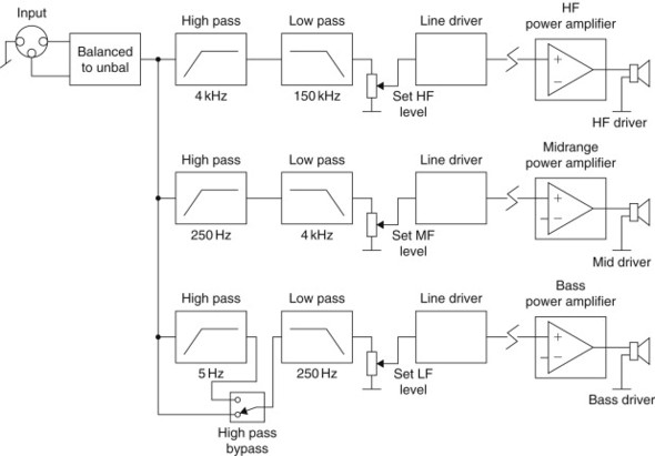
The main disadvantage of active crossover systems is cost, not just of the active crossover, but of the added amplification and cabling. In DIY domestic setups there is also the bulk of equipment (if using, say, three stereo amplifiers, placed centrally, or six mono block amps and two mono crossovers, half to be placed by each speaker) and their cabling. Such inconvenience is irrelevant in concert sound systems, and even in recording studios. It is also absent in active powered enclosures and is the rather the reverse—1 integrated active cabs are “plug in and go” systems. For everyone else, more care is needed when connecting up an active system, taking care that the drive units are going to be fed their appropriate band. In professional systems, multipin speaker and line connectors are commonly used so that the two or more frequency bands’ connections are always routed correctly.

Notable advantages compared to the common, high-level passive crossover are:

1. Reduced “congestion” and similar intermodulation distortion symptoms as each power amplifier handles only a section of the audio range.
2. Differences in driver sensitivities (considered under “matching levels,” see earlier discussion) are ironed out and without compromise, except the requirement for, or use of amplifier headroom, by simply adjusting gain controls.
3. Higher dynamic headroom by diversity, as the program peaks occurring in the respective out-of-band frequency ranges do not steal any headroom. Also, brief clipping (overdrive) of the bass band (etc.) has little effect on clarity when the other bands are not driven into clipping at the same time.
4. Amplifiers are connected directly to their respective drive-unit(s). There are no reactive components (i.e., the passive crossover) to steal current, but the drive-unit’s impedance dips may still demand significant current headroom from the amplifier.
5. The ease and capability of creating highly conjugate, highly matched, and closely toleranced crossover functions.

Of these, the low-level passive crossover potentially has all the same advantages—except possibly this last item.

24.1.4.8. Active Manifestations

Active crossovers commonly take one of three forms. In pro-audio, “the crossover” is commonly used packaged in its own box, like other signal processors, as a stand alone. As a power amplifier presents a (literally) well-placed opportunity to share a box and a power supply, a few power amp makers offer a pluggable option or “octal socket,” where a crossover module or card can be retrofitted. Often, the performance of the card’s filtering (e.g., the frequency and slope rate) may be decided upon by the user. This is often a low-budget option limited to installation work, but while it can save money, it need not be shoddy. If carried out with as much care as any crossover is due, turning an amplifier into a “speaker-driving filter” has the advantage of minimizing superfluous hardware and signal path complexity.

Otherwise, the active crossover, along with the power amplifiers, is placed in the loudspeaker enclosure. This creates an “active enclosure,” “active speaker,” or “Tri-amp cab” (if three way; else “bi-amped-cab,” “quad-amped-cab,” etc.) that has the advantage of hiding the complexity and offers a fait accompli, but takes away the flexibility that touring PA users often need.

Active systems are widely used in pro-audio, for installed and touring PA systems, and studio control room monitors. In nearly all cases, stand-alone active crossovers, discrete power amplifiers, and individual enclosures are brought together. In high-end hi-fi, discrete active systems are comparatively rare, except in DIY circles. Active speakers are becoming somewhat more common, at least in the United Kingdom and Europe.

24.1.4.9. Bi-wiring

Bi-wiring is a “part-way house” to having a low level active (or passive) crossover. A separate speaker connecting wire is provided for each drive unit, or for each frequency band (Figure 24.7). This lessens interaction and intermodulation that is otherwise caused by communal speaker cabling.

Figure 24.7. Bi-wiring improves sonic quality by avoiding superimposition voltage drops over the greater length of the output stage to speaker connection, as otherwise LF signal currents upset the hf’s driver signal’s purity, and even vice versa.

24.1.4.10. Other Networks

Whether the crossover is passive and high level, passive and low level, or active, other components may be associated with each drive unit:

1. DC protection capacitors are connected in series with drive-units to block steady current flow should a DC voltage appear across the box’s, the speaker’s, or the driver’s input terminals. They are not required for hf (and mf) drivers with passive crossovers, where the high and “bandpass” filters already include the required series capacitor as part of the crossover.

In some designs, more complex, active crowbar circuitry is used, in order to obviate the need for a series capacitor.

2. Zobel and other “conjugate matching” networks. Comprising networks of capacitors and resistors, and less often inductors, these act to smooth out the impedance variations of the drive-units, either singly or altogether, and as seen by the preceding crossover and also amplifier.

3. Music overdrive protection—in some designs, a light bulb, usually a rugged 12-V type, is connected in series with hf drive units, which in practice require protection most of all. At worst, the light bulb will be quicker, easier and less expensive to change than the hf driver or diaphragm. The effect the light bulb has on sonic quality can be small and sonically benign if the lamp is not visibly glowing during normal loud passages. “Auto resetting” “thermal trip devices,” alias Ptc (positive temperature coefficient) thermistors, are also used. These are usually in the form of a cement-coated disc. At room temperature, they exhibit a low resistance. When eventually tripped by excess current, the hot resistance increases rapidly to about 100-fold, and the protected driver’s power dissipation drops 10,000-fold ox pro-rata. The effects on sonic quality of series ptc thermistors are as yet questionable.

24.1.4.11. Other Protection

Loudspeakers have also been protected by add-on boxes, containing historic power-reading circuitry, for example, which crudely opens a relay in line with the speaker or line level signal if the drive-unit is seen heading toward a burnout.

24.2. The Interrelation of Components

24.2.1. What Loudspeakers Look Like to the Amplifier

There is a tacit presumption that most amplifiers can comfortably drive any “reasonable” loudspeaker. Beyond whatever is “reasonable,” discomfort may occur to all parties. To the power amplifier, which is nothing but a loudspeaker driver, the most salient information about any loudspeaker it is expected to drive, and the stress that may engender, is that loudspeaker’s impedance.

24.2.1.1. Impedances

A speaker’s nominal impedance is commonly (and oversimplistically) described by a single round figure, usually 15, 8, or 4 ohms for the majority of moving coil drive-units. With ribbon drive-units, or whenever several drive units are paralleled to increase handling or coverage, lower impedances of 3, 2, or 1 ohms or even less are the norm. With electrostatic and piezo (hf) drive-unit types, the load impedance can be higher, but are also more or predominantly capacitative (like a capacitor) across the audio range. This can be far more taxing to the amplifier.

24.2.1.2. Low versus High Impedances

At this juncture it is helpful for those unfamiliar with electronics jargon to grasp a counterintuitive fact: that the lower impedance, the heavier the (current) loading on the amplifier. To remember this and that 4 ohms is harder to drive than 16 ohms, think of hill slopes: a l-in-4 hill is far harder to drive or climb up than a l-in-16, that is, an impedance in ohms is the reciprocal of the relative loading. Remember also:

A low impedance demands more current, and less signal voltage is needed for a given current.

A high impedance requires more signal voltage to be driven with a given current.

24.2.1.3. Variation versus Frequency

Loudspeakers’ impedances nearly always vary over the frequency range of use. Figure 24.8 shows how a nominal 8-ohm, 15” bass drive-unit typically varies from 5.5 ohms at 450 Hz, peaking up to about 40 ohms or so, at the mechanical resonant frequency, which typically lies between 20 to 120 Hz for a bass driver. Here it is 31 Hz. Together, the drive-unit and the speaker enclosure largely determine this. Impedance also rises to a maximum at (and beyond) the highest usable frequency.

Figure 24.8. The impedance of a 15” drive unit mounted on a nominal baffle. In some cabinet designs, there could be two or more resonant peaks. Note the labeling of the resistive, capacitative, and inductive impedance zones.

At and about the resonant frequency, the impedance variation at the loudspeaker’s terminals is due to the reflection of mechanical energy storage, and damping, back to the electrical domain. Figure 24.9 shows that the loading is capacitative on the right side of the resonant peak, where impedance is falling with increasing frequency, while the impedance that slopes upward with increasing frequency, on the left side of the resonant peak, is inductive. Figure 24.9 shows this in another domain. When the phase (lower graph, left scale) is positive, the impedance is capacitative; when negative, it is inductive. When toward the center, it is resistive. Dead center is pure resistance.

Figure 24.9. The impedance of Figure 24.8 (upper graph), shown alongside the phase map (lower graph), clearly shows the relationship between pure resistance and inductive and capacitative phase—at least in terms of voltage. In some instances, a plot of current phase might be more appropriate.

The resonant frequency area(s) of any bass speaker system is are commonly highly stressful to amplifiers, and with many BJT amplifiers, when contact is prolonged by a low enough frequency and perhaps an insistently enough pounded note, it has frequently been fatal. Other amplifiers have been known to simply burst into uncontrollable oscillation.

At or above the highest usable frequency, the impedance rise is again inductive. It represents the effects of the voice coil inductance. Eddy currents, as such, or manifest as skin effect and proximity effect, may also contribute to the inductivity. Inductive effects are the cause of back EMFs (“kick back” voltages) that, unless damped, can upset sound quality and can even destroy an unsound amplifier design.

24.2.1.4. Passive Crossover Effects

Most high-performance speakers for domestic and small studio use contain passive (unpowered) crossovers. Such enclosures are driven from a single amplifier. Passive crossover networks are “in line with” the drive units’ impedances. The combination is complex; it may increase or decrease peak current demand, hence loading. As an example of the latter, extra parts may be added to create a conjugate crossover, which makes the overall loading look resistive, but also absorbs power.

24.2.1.5. Static versus Transient

Conventionally, impedance values are taken after applying a steady and repetitive test signal (e.g., continuous sine wave) and allowing a few moments for the recovered signal amplitude that represents impedance to settle. In the short term, impedance can be considerably lower. At worst, it is possible for an ordinary dynamic (moving coil) type of loudspeaker to demand current as is it had 1/6th of its nominal impedance. In other words, an 8-ohm speaker can sometimes look like 1.4 ohms. This will not happen all the time or even very often, nor for very long at a time; however, for high-quality sound reproduction, and not forgetting that music involves repetition, the possibility must be allowed for.

24.2.1.6. Acoustic Contribution

The impedance (load) characteristics of drive units can be affected by cabinet air leaks, and also by reflections in the room, hence the positioning of the enclosure. Horn-loaded drive-units are usually the most sensitive to this.

The upshot is that most loudspeaker loads are a wide variable, not just between different models and types, but depending on program dynamics and excitation frequencies.

24.2.2. What Speakers Are Looking For

The fact that most loudspeakers do not employ conjugate impedance compensation, and so they have impedance curves that vary “all over” with frequency, means that for high performance, the amplifier kind the speaker needs to see is a “voltage source.”

24.2.2.1. Why Voltage?

The signal voltage must be almost unaffected (ideally far below say 1% change) whether the speaker is connected or not, regardless of whether it’s drawing 50 milliamps or 50 amperes. That means a “stiff power source,” alias a low impedance or “high-current-capable” source.

If the source impedance isn’t low (enough), then as the speaker’s impedance varies with frequency, the change will be superimposed on its own frequency response as a tonal aberration. A source impedance that is almost as high as speakers’ own minimum impedances is a major failing with power amplifiers having low or nil global negative feedback, and the outcome is a tonal anomaly as gross as 5 dB. This may not be all bad, but it will certainly be arbitrary.

24.2.2.2. Energy Control

In part, a voltage source is required to drive speakers, because loudspeakers store, as well as convert, energy. The fundamental resonance is the place (in the frequency domain) where this is most true. Some of the stored energy “kicks back” and needs to be damped quickly (dissipated) to avoid transient distortion or “smearing.” The same reactive effects may also demand surprisingly high peak currents from the amplifier at other times, when driven by music signals.

In both cases, the answer is a high current sourcing and sinking capability. Both of these features are implied but neither are guaranteed by a low source impedance. The overall requirement is a “current-capable-enough voltage source.” So far, most power amplifiers throughout history have aimed to be this, but some have come closer than others.

24.2.2.3. Damping Factor?

The majority of high-performance amplifiers are solid state and employ global (overall) negative feedback, not least for the unit-to-unit consistency it offers over the wild (e.g., +/−50%) tolerances of semiconductor parts. One effect of high global NFB (in conventional topologies) is to make the output source impedance (Z⁰) very low, potentially 100 times lower than the speaker impedance at the amplifier’s output terminals. For example, if the amplifier’s output impedance is 40 wohms, then the nominal damping factor with an 8-ohm speaker will be 200, that is, 40 milliohms (0.04) is l/200th of 8 Q. This “damping factor” is essential for the accurate control of most speakers.

Yet describing an amplifier’s ability to damp a loudspeaker with a single number (called “damping factor”) is doubtful. This is true even in active systems where there is no passive crossover with their own energy storage effects, complicating especially dynamic behavior.

Figure 24.10 again takes a sine-swept impedance of an 8-ohm, 15” driver in a nominal box to show how “static” speaker damping varies. Impedance is 70 ohms at resonance but 5.6 ohms at 450 Hz. The bottom part of Figure 24.10 plots the output impedance of a power amplifier that has high negative feedback, and thus the source impedance looking up (or into) it is very low (6 milliohms at 100 Hz), although increasing monotonically above 1 kHz. The traditional, simplistic “damping factor” takes this ideal impedance at a nominal point (say 100 Hz) and then describes attenuation against an 8-ohm resistor. This gives a damping factor of about three orders, that is, 1000, but up to 10,000 at 30 Hz. Now look at the middle curve of Figure 24.10. This is what the amplifier’s damping ability is degraded to, after it has traversed a given speaker cable and passed through an ideal 10,000-μF series capacitor, as fitted commonly in many professional cabinets for belt’ n’ braces DC fault protection. The rise at 1 kHz is due to cable resistance, while cable inductance and series capacitance cause the high- and low-end rises, respectively, above 100 milliohms.

Figure 24.10. Views of the damping surface in 2D. The lower plot shows the very low steady-state output source impedance of a typical transistor amplifier with high NFB. The middle plot shows how this degrades after passing down a few meters of reasonably rated cable and a series capacitor (which might be the simplest crossover, or for fault protection). The upper plot repeats the impedance versus frequency behavior of the 15” bass driver. The effective damping factor is the smaller and highly variable difference between the upper and the middle plots, not the difference between the highest impedance on the upper plot and the lowest on the lower plot used by amplifier makers!

We can easily read off static damping against frequency: at 30 Hz, it’s about ×l00. At midfrequencies, it’s about ×50, and again about 100 at 10 kHz. However, instantaneous “dynamic” impedance may dip four times lower, while the DC resistance portion of the speaker impedance increases after hard drive, recovering over tens to thousands of milliseconds, depending on whether the drive-unit is a tweeter or a 240” shaker.

Even with high NFB, an amplifier’s output impedance will be higher with fewer output transistors, less global feedback, junction heating (if the transistors doing the muscle work are MOS-FETs), and more resistive or inductive (longer/thinner) cabling. Reducing the series DC protection capacitor value so it becomes a passive crossover filter will considerably increase source impedance, even in the pass band. The ESR (losses) of any series capacitors and inductors will also increase source impedance, with small, but complex nested variations with drive, temperature, use patterns, and aging. The outcome is that the three curves—and the difference between the upper two that is the map of damping factor—writhe unpredictably.

Full reality is still more complex, as all loudspeakers comprise a number of complex energy storage/release/exchange sections, some interacting with the room space, and each with the others. The conclusion is that damping factor has more dimensions than one number can convey.

24.2.2.4. Design Interaction

While high-performance loudspeakers are being designed and optimized, and certainly before they are finalized for production, in-depth listening is a prerequisite. This means that amplifiers are required to drive them while they are being tested and optimized in thedesign process. Many drive-unit and speaker manufacturers are limited (or limit themselves) to using just one amplifier make to test their designs and production. The situation is rarely publicized.

It follows that many loudspeakers are inevitably looking for that one kind of amplifier that was used when they were “voiced” and “tweaked” by their designer(s). With no less potential for habitual patterns, listeners are looking for the amp that interacts with a loudspeaker in a particular way. The combined behavior or “chemistry” is complex and can be unpredictable and frustratingly unrelated to the type or class of amplifier.

Here is just one reason why the ideal high-performance power amplifier/speaker combination can be determined only by trying them together and why quite disparate amplifier designs and topologies may shine equally through a particular speaker.

Knowledgeable “high-end” loudspeaker designers and manufacturing companies employ a well-chosen group of different power amplifiers. One or two will be the best sounding “references”; some will be widely used models and not particularly good performers; others will be niche models, discovered accidentally over the years, that expose loudspeaker problems.

24.2.3. What Passive Crossovers Look Like to Amplifiers

For conventional full-range loudspeakers with passive crossovers, the crossover components stand between the amplifier and the speaker. Unless the speaker’s drive unit(s) is/are blown or have been disconnected or removed, then the crossover won’t usually be “seen electrically” (by the amplifier) on its own. Figure 24.11 shows the impedance that would be seen by the power amplifier if the loudspeakers were 8-ohm resistors and how it drops from about 10.5 ohms to just over 5 ohms at the crossover point. As both drivers are being driven at this point, it’s what you might expect. Figure 24.12 shows how much the picture changes when the resistors are replaced by real speakers: now there are two dips.

Figure 24.11. If speakers were simply resistors, the load on the amplifier might appear as here, with the apparent 11-ohm load simply halving to 5.5 ohms at the one point where the two drivers are both drawing substantial current, the crossover point. Note that the crossover dip may as well be a resonance and, as such, adds to the amplifier’s load stress.

Figure 24.12. Here, the resistors are replaced by drive-units having the impedance characteristics shown in the lower graph. The upper graph shows how the impedance seen by the amplifier has changed—notably two dips where there was one.

In the crossover’s pass band where there should be no (attenuative) action on the signal voltage at all, the crossover should be “transparent.” In practice, one pass band is another driver’s stop band. Even a steady-state test signal will experience the added reactive loading at most frequencies. In turn, the crossover is liable to add to the peak current demanded by the drive-units. With music signals, a passive crossover stores energy and can “kick back” like a speaker, potentially adding to the speaker’s demands. Overall, for the amplifier’s own good, passive crossovers benefit no less than the drive unit from being coupled to an amplifier with very low source impedance, with ample current sourcing and sinking capability.