Chapter 2. Measurement

2.1. Concepts Underlying the Decibel and its Use in Sound Systems

Most system measurements of level start with a voltage amplitude. Relative level changes at a given point can be observed on a voltmeter scale when it is realized that(2.1)

which is only true if both values are measured at an identical point in their circuit. A common usage has been to remove the exponent from the ratio and apply it to the multiplier.(2.2)

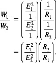
Bear in mind that the decibel is always and only based on a power ratio. Any other kind of ratio (i.e., voltage, current, or sound pressure) must first be turned into a power ratio by squaring and then converted into a power level in decibels.

2.1.1. Converting Voltage Ratios to Power Ratios

Many audio technicians are confused by the fact that doubling the voltage results in a 6-dB increase while doubling the power only results in a 3-dB increase. Figure 2.1 demonstrates what happens if we simultaneously check both the voltage and the power in a circuit where we double the voltage. Note that for a doubling of the voltage, the power increases four times.(2.3)

(2.4)

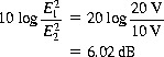
Figure 2.1. Voltage and power relationships in a circuit.

2.1.2. The dBV

One of the most common errors when using the decibel is to regard it as a voltage ratio (i.e., so many decibels above or below a reference voltage). To compound the error, the result is referred to as a “level.” The word “level” is reserved for power; an increase in the voltage magnitude is properly referred to as “amplification.”

However, the decibel can be legitimately used with a voltage reference. The reference is 1.0 V. When voltage magnitudes are referenced logarithmically, they are called dBV (i.e., dB above or below 1.0 V). This use is legitimate because all such measurements are made open circuit and can easily be converted into power levels at any impedance interface.

The following definition is from the IEEE Standard Dictionary of Electrical and Electronics Terms, Second Edition:

2.1.2.1. 244.62

Voltage Amplification (1) (general). An increase in signal voltage magnitude in transmission from one point to another or the process thereof. See also: amplifier. 210 (2) (transducer). The scalar ratio of the signal output voltage to the signal input voltage. Warning: By incorrect extension of the term decibel, this ratio is sometimes expressed in decibels by multiplying its common logarithm by 20. It may be currently expressed in decilogs. Note: If the input and/or output power consist of more than one component, such as multifrequency signal or noise, then the particular components used and their weighting must be specified. See also: Transducer.

2.1.2.2. 239.210

Decilog (dg). A division of the logarithmic scale used for measuring the logarithm of the ratio of two values of any quantity. Note: Its value is such that the number of decilogs is equal to 10 times the logarithm to the base 10 of the ratio. One decilog therefore corresponds to a ratio of 10^0.1 (that is 1.25829+).

2.1.3. The Decibel as a Power Ratio

Note that 20 W/10 W and 200 W/100 W both equal 3.01 dB, which means that a 2 to 1 (2:1) power ratio exists but reveals nothing about the actual powers. The human ear hears the same small difference between 1 and 2 W as it does between 100 and 200 W.

Changing decibels back to a power ratio (exponential form) is the same as for any logarithm with the addition of a multiplier (Figure 2.2). The arrows in Figure 2.2 indicate the transposition of quantities. Table 2.1 shows the number of decibels corresponding to various power ratios.

Figure 2.2. Conversion of dB from logarithmic form to exponential form.

Table 2.1. Power Ratios in Decibels

Power ratio	Decibels (dB)
2	3.01030
3	4.77121
4	6.02060
5	6.98970
6	7.78151
7	8.45098
8	9.03090
9	9.54243
10	10.00000
100	20.00000
1000	30.00000
10,000	40.00000
100,000	50.00000
1,000,000	60.00000

2.1.4. Finding Other Multipliers

Occasionally in acoustics, we may need multipliers other than 10 or 20. Once the ΔdB (the number of dB for a 2:1 ratio change) is known, calculate the multiplier by(2.5)

For example, if a 2:1 change is equivalent to 3.01 dB, then(2.6)

or

10log2=3.01.

If a 2:1 change is equivalent to 6.02 dB, then

or

20log2=6.02.

Finally, if a 2:1 change is equivalent to 8 dB, then

or

26.58 2log=8.

For any ΔdB corresponding to a 2:1 ratio change involving logarithms to the base 10, this may be reduced to(2.7)

2.1.5. The Decibel as a Power Quantity

We have seen that a number of decibels by themselves are only ratios. Given any reference (such as 50 W), we can use decibels to find absolute values. A standard reference for power in audio work is 10⁻³ W (0.001 W) or x V across Z Ω. Note that when a level is expressed as a wattage, it is not necessary to state an impedance, but when it is stated as a voltage, an impedance is mandatory. This power is called 0 dBm. The small “m” stands for milliwatt (0.001 W) or one-thousandth of a watt.

2.1.6. Example

The power in watts corresponding to +30 dBm is calculated as follows:

For a power of −12 dBm:

The voltage across 600 Ω is

Note that this −12-dBm power level can appear across any impedance and will always be the same power level. Voltages will vary to maintain this power level. In constant-voltage systems the power level varies as the impedance is changed. In constant-current systems the voltage changes as the impedance varies (i.e., −12 dBm across

2.2. Measuring Electrical Power

(2.8)

(2.9)

where W is the power in watts, E is the electromotive force in rms volts, I is the current in rms amperes, Z is the magnitude of the impedance in ohms [in audio (AC) circuits Z (impedance) is used in place of R (AC resistance)], and θ is the phase difference between E and I in degrees.

These equations are only valid for single frequency rms sine wave voltages and currents.

2.2.1. Most Common Technique

1. Measure Z and θ.
2. Measure E across the actual load Z so that

2.3. Expressing Power as an Audio Level

The reference power is 0.001 W (1 mW). When expressed as a level, this power is called 0 dBm (0 dB referenced to 1 mW).

Thus to express a power level we need two powers—first the measured power W¹ and second the reference power W². This can be written as a power change in dB:(2.10)

This can be written as a power level:(2.11)

or(2.12)

2.3.1. Special Circumstance

When R¹=R² and only then:(2.13)

where E² is the voltage associated with the reference power.

2.4. Conventional Practice

When calculating power level in dBm, we commonly make E²=0.775 V and R²=600 Ω. Note that E² may be any voltage and R² any resistance so long as together they represent 0.001 W.

2.4.1. Levels in dB

when R¹=R²

1. The term “level” is always used for a power expressed in decibels.

2. 

1. Power definitions:
   • Apparent power=E×I or E²⁄Z,
   • The average real or absorbed power is (E²⁄Z)cosθ,
   • The reactive power is (E²⁄Z)sinθ,
   • Power factor=cosθ.
2. The term “gain” or “loss” always means the power gain or power loss at the system’s output due to the device under test.

2.4.2. Practical Variations of the dBm Equations

When the reference is the audio standard, that is, 0.77459 V and 600 Ω, then(2.14)

where E²=0.77459 ... V, R²=600 Ω. Then

and 1/1000=0.001. Note that any E² and R² that result in a power of 0.001 W may be used. We can then write:(2.15)

and(2.16)

See Figure 2.3.

Figure 2.3. Power in dB across a load versus available input power.

For all of the values in Table 2.2 the only thing known is the voltage. The indication is not a level. The apparent level can only be true across the actual reference impedance. Finally, the presence or absence of an attenuator or other sensitivity control is not known. See Section 2.20 for an explanation of VU.

Table 2.2. Root Mean Square Voltages Used as Nonstandard References

Voltage (V)	Meter indication	Apparent level (VU)	User
1.950	0	+8	Broadcast
1.230	0	+4	Recording
0.245	0	−10	Home recording
0.138	0	−15	Musical instruments

The power output of Boulder Dam is said to be approximately 3,160,000,000 W.Expressed in dBm, this output would be

2.5. The Decibel in Acoustics—L^P, L^W, and L^I

In acoustics, the ratios encountered most commonly are changes in pressure levels. First, there must be a reference. The older level was 0.0002 dyn/cm², but this has recently been changed to 0.00002 N/m² (20 μN/m²). Note that 0.0002 dyn/cm² is exactly the same sound pressure as 0.00002 N/m². Even more recently the standards group has named this same pressure pascals (Pa) and arranged this new unit so that(2.17)

This means that if the pressure is measured in pascals,(2.18)

If the pressure is measured in dynes per square centimeter (dyn/cm²), then(2.19)

The root mean square (rms) sound pressure P can be found by(2.20)

where P^rms is in pascals, f is the frequency in Hertz (Hz), A is particle displacement in meters (rms value), ρ is the density of air in kilograms per cubic meter (kg/m³), c is the velocity of sound in meters per second (m/s), ρc=406 RAYLS and is called the characteristic acoustic resistance (this value can vary), or(2.21)

These are identical sound pressure levels bearing different labels. Sound pressure levels were identified as dB-SPL, and sound power levels were identified as dB-PWL. Currently, L^P is preferred for sound pressure level and L^W for sound power level. Sound intensity level is L^I:(2.22)

At sea level, atmospheric pressure is equal to 2116 1b/ft². Remember the old physics laboratory stunt of partially filling an oil can with water, boiling the water, and then quickly sealing the can and putting it under the cold water faucet to condense the steam so that the atmospheric pressure would crush the can as the steam condensed, leaving a partial vacuum?

1Atm=101,300 PaTherefore

This represents the complete modulation of atmospheric pressure and would be the largest possible sinusoid. Note that the sound pressure (SP) is analogous to voltage. An L^P of 200 dB is the pressure generated by 50 lb of TNT at 10 ft. Table 2.3 shows the equivalents of sound pressure levels.

Table 2.3. Equivalents of Pressure Levels

Older values of a similar nature are:

1 microbar ≅ 1/1,000,000 of atmospheric pressure

≅74 dB

therefore

1 Pa=10 dyn/cm2

Other interesting figures:

Atmospheric pressure fully modulated LP ≅ 194 dB

1 lb/ft2LP=127.6 dB

1 lb/in2LP=170.8 dB

50 lb of TNT measured at 10 ft LP=200 dB

12-inch cannon, 12 ft in front of and below muzzle LP

=220+dB

Courtesy of GenRad Handbook.

For additional insights into these basic relationships, the Handbook of Noise Measurement by Peterson and Gross is thorough, accurate, and readable.

2.6. Acoustic Intensity Level (L^I), Acoustic Power Level (L^W), and Acoustic Pressure Level (L^P)

2.6.1. Acoustic Intensity Level, L^I

The acoustic intensity I^a (the acoustic power per unit of area—usually in W/m² or W/cm²) is found by(2.23)

2.6.2. Acoustic Power Level, L^W

The total acoustic power can also be expressed as a level (L^W):(2.24)

2.6.3. Acoustic Pressure Level, L^P

To identify each of these parameters more clearly, consider a sphere with a radius of 0.282 m. (Since the surface area of a sphere equals 4πr², this yields a sphere with a surface area of 1 m².) An omnidirectional point source radiating one acoustic watt is placed into the center of this sphere. Thus we have, by definition, an acoustic intensity at the surface of the sphere of 1 W/m². From this we can calculate the P^rms:(2.25)

where W^a is the total acoustic power in watts and ρc equals 406 RAYLS and is called the characteristic acoustic resistance.

Knowing the acoustic watts, P^rms is easy to find:

Thus the L^P must be

and the acoustic power level in L^W must be

Thus the L^P, L^I, and L^W at 0.282 m are the same numerical value if the source is omnidirectional (see Figure 2.4).

Figure 2.4. Relationship of spherical surface area to radius.

2.7. Inverse Square Law

If we double the radius of the sphere to 0.564 m, the surface area of the sphere quadruples because the radius is squared in the area equation (A=4πr²). Thus our intensity will drop to one-fourth its former value. (Note, however, that the total acoustic power is still 1 W so the L^W still is 120 dB.) Now an intensity change from 1 W to 0.25 W/m² can be written as a decibel change. The acoustic intensity (i.e., the power per unit of area) has dropped 6 dB in any given area:

Therefore our L^P had to also drop 6 dB and would now be approximately 114 dB.

This effect is commonly called the inverse square law change in level. Gravity, light, and many other physical effects exhibit this rate of change with varying distance from a source. Obviously, if you halve the radius, the levels all rise by 6 dB.

2.8. Directivity Factor

Finally, make the point source radiating one acoustic watt a hemispherical radiator instead of an omnidirectional one. Thus at 0.282 m the surface area is now half of what our sphere had or 0.5 m². Therefore our intensity is now 1 W/0.5 m² or the equivalent 2 W/m²:

Therefore our L^P is 123.01 dB. L^w remains 120 dB.This 3.01-dB change represents a 2:1 change in the power per unit area; thus, a hemispherical radiator is said to have twice the directivity factor a spherical radiator has. The directivity factor is identified by a number of symbols—D^F , Q, Rθ, λ, M, etc. Q is the most widely used in the United States so we have chosen it for this text. Directivity can also be expressed as a solid angle in steradians or sr=4π/Q.

2.9. Ohm’s Law

Recall that the use of the term “decibel” always implies a power ratio. Power itself is rarely measured as such. The most common quantity measured is voltage. If in measuring the voltage of a sine wave signal (oscillators are the most reliable and common of the test-signal sources) you obtain the rms voltage, you can calculate the average power developed by using Ohm’s law. Figure 2.5 is a reminder of its many basic forms and uses the following definitions:

• W is the average electrical power in watts (W).
• I is the rms electrical current in amperes (A).
• R is the electrical resistance in ohms (Ω).
• E is the electromotive force in rms volts (V).
• PF is the power factor (cosθ).

Figure 2.5. Ohm’s law nomograph for AC or DC.

2.10. A Decibel is a Decibel is a Decibel

The decibel is always a power ratio; therefore, when dealing with quantities that are not power ratios, that is, voltage, use the multiplier 20 in place of 10. As we encounter each reference for the dB, we will indicate the correct multiplier. Table 2.4 lists all the standard references, and Tables 2.5 through 2.8 contain additional information regarding reference labels and quantities. The decibel is not a unit of measurement like an inch, a watt, a liter, or a gram. It is the logarithm of a nondimensional ratio of two power-like quantities.

Table 2.4. Common Decibel Notations and References

Quantity	Standard reference	Symbol	Log multiplier
Sound pressure	Water: 1 dyn/cm2	SPL or	20
	Air: 0.0002 dyn/cm2	LP
	or 0.00002 N/m2
Sound intensity	10−16 W/cm2		10
	10−12 W/m2
Sound power	10−12 W (new)	PWL	10
	10−13 W (old)	or Lw
Audio power	10−3 W	dBm	10
EMF	1 V	dBV	20
Amperes	1 mA		20
Acceleration	1 gRMS		20
Acceleration	1 g2/Hz		10
Spectral density
Volume units	10−3 W	VU	10
Distance	1 ft or 1 m	ΔDx	20
Noise-ref	−90 dBm at 1 kHz	dBm	10

Table 2.5. Preferred Reference Labels for Acoustic

Name	Definition
Sound pressure squared level	LP=20 log (p/po) dB
Vibratory acceleration level	La=20 log (a/ao) dB
Vibratory velocity level	LV=20 log (v/vo) dB
Vibratory force level	LF=20 log (F/Fo) dB
Power level	LW=10 log (P/Po) dB
Intensity level	LI=10 log (I/Io) dB
Energy density level	LE=10 log (E/Eo) dB

Table 2.6. A-Weighted Recommended Descriptor List

Term	Symbol
A-weighted sound level	LA
A-weighted sound power level	LWA
Maximum A-weighted sound level	Lmax
Peak A-weighted sound level	L pk
Level exceeded 3% of the time	Lx
Equivalent sound level	Leq
Equivalent sound level over time (T)	Leq(T)
Day sound level	Ld
Night sound level	Ln
Day–night sound level	Ldn
Yearly day–night sound level	Ldn(Y)
Sound exposure level	LSE

Table 2.7. Associated Standard Reference Values

1 atm=1.013 bar=1.033 kpa/cm2=14.70 lb/in2=760 mm Hg=29.92 in Hg

Acceleration of gravity: g=980.665 cm/s2=32.174 ft/s2 (standard or accepted value)

Sound level: The common reference level is the audibility threshold at 1000 Hz, i.e., 0.0002 dyn/cm2, 2×1024 μbar, 2×10−5 N/m2, 10−16 W/cm2

Table 2.8. Recommended Descriptor List

Term	A weighting	Alternativea A weighting	Other weightingb	Unweighted
Sound (pressure) levelc	LA	LpA	LB, LpB	LP
Sound power level	LWA		LWB	LW
Maximum sound level	Lmax	LAmax	LBmax	Lpmax
Peak sound (pressure) level	LApk		LBpk	Lpk
Level exceeded x% of the time	Lx	LAx	LBx	LPx
Equivalent sound level	Leq	L Aeq	LBeq	Lpeq
Equivalent sound level over time (T)d	Leq(T)	LAeq(T)	LBeq(T)	Lpeq(T)
Day sound level	Ld	LAd	LBd	Lpd
Night sound level	Ln	LAn	LBn	Lpn
Day–night sound level	Ldn	LAdn	LBdn	Lpdn
Yearly day–night sound level	Ldn(Y)	LAdn(Y)	LBdn(Y)	Lpdn(Y)
Sound exposure level	LS	LSA	LSB	LSp
Energy average value over (nontime domain) set of observations	Leq(e)	LAeq(e)	LBeq(e)	Lpeq(e)
Level exceeded x% of the total set of (nontime domain) observations	Lx(e)	LAx(e)	LBx(e)	Lpx(e)
Average Lx value	Lx	LAx	LBx	Lpx

^a “Alternative” symbols may be used to assure clarity or consistency.

^b Only B weighting is shown. Applies also to C, D, and E weighting.

^c The term “pressure” is used only for the unweighted level.

^d Unless otherwise specified, time is in hours [e.g., the hourly equivalent level is L^eq(1)]. Time may be specified in nonquantitative terms [e.g., could be specified as L^eq(WASH) to mean the washing cycle noise for a washing machine].

For L^P=20 log (x Pa/0.00002 Pa), use Eq. (2-29).(2.26)

2.11. Older References

Much earlier, but valuable, literature used 10⁻¹³ W as a reference. In that case, the L^P value approximately equals the L^W value at 0.282 ft from an omnidirectional radiator in a free field (i.e., the number values are the same but, of course, different quantities are being measured). For 1 W using 10⁻¹² W at 0.283 m, L^W ≅ L^P=120 dB. For 1 W using 10⁻¹³ W at 0.282 ft, L^W ≅ L^P=130 dB as found with the equation:(2.27)

where L^W is 10 log the wattage divided by the reference power 10⁻¹³ and r is the distance in meters from the center of the sound source.

Figure 2.6 requires that you either know the distance from the source or assumes you are in the steady reverberant sound field of an enclosed space. L^P readings without one of these is meaningless.

Figure 2.6. Typical A-weighted sound levels as measured with a sound level meter. (Courtesy of GenRad.)

Figure 2.7 shows typical power and L^W values for various acoustic sources.

Figure 2.7. Typical power and L^W values for various acoustic sources.

2.12. The Equivalent Level (L^EQ) in Noise Measurements

Increasingly, acoustical workers in the noise control field are erecting an interesting edifice of measurement systems. A number of these measurement systems are based on the concept of average energy. Suppose, for example, that we have some means of collecting all of the A-weighted sound energy that arrives at a particular location over a certain period of time such as 90 dBA for 3.6 s (this could be a series of levels that lasted seconds, hours, or even days). We can then calculate the decibel level of steady noise for, say, 1 h that would be the equivalent level of the dBA for 3.6 s. That is, we wish to find the energy equivalent level for 1 h:(2.28)

where P^A is the acoustic pressure, P^o is the reference acoustic pressure, and 3600 s is the averaging time interval.

This integration reduces to

Thus 1.0 hour of noise energy at 60 dBA is the equivalent energy exposure of 90 dBA for 3.6 s.

L^DN (day–night level), CNEL (community noise level), and so on all follow similar schemes with variation in weightings for differing times of day, etc.

It is of interest that shooting a 0.458 magnum 174.7 L^P (peak) for 2.5 ms translates into

of steady sound for 1 h. OSHA allows only 15 min of exposure to levels of 110–115 dBA. As Howard Ruark’s African guide, Harry Selby, remarked after Ruark had accidentally set off both barrels at once of a 0.470 express rifle while being charged by a Cape buffalo, “One of you ought to get up.”

2.13. Combining Decibels

2.13.1. Adding Decibel Levels

The sum of two or more levels expressed in dB may be found as follows:(2.29)

If, for example, we have a noisy piece of machinery with an L^P=90 dB and wish to turn on a second machine with an L^P=90 dB, we need to know the combined L^P. Because both measured levels are the result of the power being applied to the machine, with some percentage being converted into acoustic power, we can determine L^T by using Eq. (2-33). Therefore

Doubling the acoustic power results in a 3 dB increase.

An alternative dB addition technique is given through the courtesy of Gary Berner.(2.30)

Example

If we wish to add 90 dB to 96 dB, using Eq. (2-33), take the difference in dB (6 dB) and put it in the equation:

Input signals to a mixing network also combine in this same manner, but the insertion loss of the network must be subtracted. Two exactly phase-coherent sine wave signals of equal amplitude will combine to give a level 6 dB higher than either sine wave.

The general case equation for adding sound pressure, voltages, or currents is(2.31)

Table 2.9 shows the effects of adding two equal amplitude signals with different phases together using Eq. (2-36).

Table 2.9. Combining Pure Tones of the Same Frequency but Differing Phase Angles

Signal 1 amplitude, LP (dB)	Signal 1 phase, in degrees	Signal 2 amplitude, LP (dB)	Signal 2 phase, in degrees	Combined signal amplitude, LP (dB)
90	0	+90	0	96.02
90	0	+90	10	95.99
90	0	+90	20	95.89
90	0	+90	30	95.72
90	0	+90	40	95.48
90	0	+90	50	95.17
90	0	+90	60	94.77
90	0	+90	70	94.29
90	0	+90	80	93.71
90	0	+90	90	93.01
90	0	+90	100	92.18
90	0	+90	110	91.19
90	0	+90	120	90.00
90	0	+90	130	88.54
90	0	+90	140	86.70
90	0	+90	150	84.28
90	0	+90	160	80.81
90	0	+90	170	74.83
90	0	+90	180	−∞

2.13.2. Subtracting Decibels

The difference of two levels expressed in dB may be found as follows:(2.32)

2.13.3. Combining Levels of Uncorrelated Noise Signals

When the sound level of a source is measured in the presence of noise, it is necessary to subtract out the effect of the noise on the reading. First, take a reading of the source and the noise combined (L^S+N). Then take another reading of the noise alone (the source having been shut off). The second reading is designated L^N. Then(2.33)

To combine the levels of uncorrelated noise signals we can also use the chart in Figure 2.8.

Figure 2.8. Chart used for determining the combined level of uncorrelated noise signals.

2.13.4. To Add Levels

Enter the chart with the numerical difference between the two levels being added (top of chart). Follow the line corresponding to this value to its intersection with the curved line and then move left to read the numerical difference between the total and larger levels. Add this value to the larger level to determine the total.

Example

To add 75 dB to 80 dB, subtract 75 dB from 80 dB; the difference is 5 dB. In Figure 2.8, the 5-dB line intersects the curved line at 1.2 dB on the vertical scale. Thus the total value is 80 dB+1.2 dB, or 81.2 dB.

2.13.5. To Subtract Levels

Enter the chart in Figure 2.8 with the numerical difference between the total and larger levels if this value is less than 3 dB. Enter the chart with the numerical difference between the total and smaller levels if this value is between 3 and 14 dB. Follow the line corresponding to this value to its intersection with the curved line and then either left or down to read the numerical difference between total and larger (smaller) levels. Subtract this value from the total level to determine the unknown level.

Example

Subtract 81 dB from 90 dB; the difference is 9 dB. The 9-dB vertical line intersects the curved line at 0.6 dB on the vertical scale. Thus the unknown level is 90 dB – 0.6 dB, or 89.4 dB.

2.14. Combining Voltage

To combine voltages, use the following equation:(2.34)

where E^T is the total sound pressure, current, or voltage; E¹ is the sound pressure, current, or voltage of the first signal; E² is the sound pressure, current, or voltage of the second signal; a¹ is the phase angle of signal one; and a² is the phase angle of signal two.

2.15. Using the Log Charts

2.15.1. The 10 Log x Chart

There are two scales on the top of the 10 log¹⁰x chart in Figure 2.9. One is in dB above and below a 1-W reference level and the other is in dBm (reference 0.001 W). Power ratios may be read directly from the 1-W dB scale.

Figure 2.9. The 10log¹⁰x chart.

Example

How many decibels is a 25:1 power ratio?

1. Look up 25 on the power–watts scale.
2. Read 14 dB directly above the 25.

Example

We have a 100 W amplifier but plan to use a 12-dB margin for “head room.” How many watts will our program level be?

1. Above 100 W find +50 dBm.
2. Subtract 12 dB from 50 dBm to obtain +38 dBm. Just below +38 dBm find approximately 6 W.

Example

A 100-W amplifier has 64 dB of gain. What input level in dBm will drive it to full power?

1. Above 100 W read +50 dBm.
2. +50 dBm − 64-dB gain=−14 dBm.

Example

A loudspeaker has a sensitivity of L^P=99 dB at 4 ft with a 1-W input. How many watts are needed to have an L^P of 115 at 4 ft?

1. 115 L^P – 99 L^P=+16 dB.
2. At +16 on the 1-W scale read 39.8 W.

2.15.2. The 20 Log x Chart

Refer to the chart in Figure 2.10. A 2:1 voltage, distance, or sound pressure change is found by locating 2 on the ratio or D scale and looking directly above to 6 dB.

Figure 2.10. The 20log¹⁰x chart.

Example

A loudspeaker has a sensitivity of L^P=99 dB at 4 ft with 1 W of input power. What will the level be at 100 ft?

1. Find the relative dB for 4 ft (relative dB=12 dB).
2. Find the relative dB for 100 ft (relative dB=40 dB).
3. Calculate the absolute dB (40 dB – 12 dB=28 dB).
4. L^P=99 dB – 28 dB=71 dB.

Example

If we raise the voltage from 2 to 10 V, how many decibels would we increase the power?

1. Find the relative dB for a ratio of 2 (relative dB=6 dB).
2. Find the relative dB for a ratio of 10 (relative dB=20 dB).
3. Absolute dB change=20 dB – 6 dB=14 dB.
4. Because a dB is a dB, the power also changed by 14 dB.

2.16. Finding the Logarithm of a Number to Any Base

In communication theory, the base 2 is used. Occasionally, other bases are chosen. To find the logarithm of a number to any possible given base, write(2.35)

where x is the number for which a logarithm is to be found, b is the base, and n is the logarithm.

Then write(2.36)

and(2.37)

Suppose we want to find the natural logarithm of 2 (written ln 2). The base of natural logarithms is e=2.7188281828. Then

To verify this result,

To find log 2 of 26,

The general case is(2.38)

2.17. Semitone Intervals

Suppose that we need

(the semitone interval in music). We could write(2.39)

Therefore

This is the same as multiplying 1.05946 by itself 12 times to obtain 2.

10^0.02508 is called the antilog of 0.02508. The antilog is also written as log⁻¹, antilog 10, or 10 exp. All these terms mean exactly the same thing.

2.18. System Gain Changes

Imagine a noise generator driving a power amplifier and a loudspeaker (Figure 2.11). If the voltage out of the noise generator is raised by 6 dB, what happens?

Voltage	Electrical power	LP	LW
Doubled	Quadrupled	Doubled	Quadrupled
+6 dB	+6 dB	+6 dB	+6 dB

Figure 2.11. Voltage, electrical power, P^w, and sound pressure compared.

This means that, in a linear system, a level change ahead of any components results in a level change for that same signal in all subsequent components, although it might be measured as quite different voltages or wattages at differing points. The change in level at any point would be the same. We will work with this concept a little later when we plot the gains and losses through a total system.

2.19. The VU and the Volume Indicator Instrument

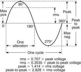
Volts, amperes, and watts can be measured by inserting an appropriate meter into the circuit. If all audio signals were sine waves, we could insert a dBm meter into the circuit and get a reading that would correlate with both electrical and acoustical variations. Unfortunately, audio signals are complex waveforms and their rms value is not 0.707 times peak but can range from as small as 0.04 times peak to as high as 0.99 times peak (Figure 2.12). To solve this problem, broadcasting and telephone engineers got together in 1939 and designed a special instrument for measuring speech and music in communication circuits. They calibrated this new type of instrument in units called VU. The dBm and the VU are almost identical; the only difference is their usage. The instrument used to measure VU is called the volume indicator (VI) instrument. (Some users ignore this and incorrectly call it a VU meter.) Both dBm meters and volume indicator instruments are specially calibrated voltmeters. Consequently, the VU and dBm scales on these meters give correct readings only when the measurement is being made across the impedance for which they are calibrated (usually 150 or 600 Ω). Readings taken across the design impedance are referred to as true levels, whereas readings taken across other impedances are called apparent levels.

Figure 2.12. Sine wave voltage values. The average voltage of a sine wave is zero.

Apparent levels can be useful for relative frequency response measurements, for example. When the impedance is not 600 Ω, the correction factor of 10 log (600/new impedance) can be added to the formula containing the reference level as in the following equation:(2.40)

The result is the true level.

2.19.1. The VU Impedance Correction

When a VI instrument is connected across 600 Ω and is indicating 0 VU on a sine wave signal, the true level is 4 dB higher, or +4 dBm, instead of 0 dBm or zero level. The reason this is so is shown in Figure 2.13. The VI instrument uses a 50-μA D’Arsonval movement in conjunction with a copper-oxide bridge-type rectifier. The impedance of the instrument and rectifier is 3900 Ω. To minimize its effect when placed across a 600-Ω line, it is “built out” an additional 3600 Ω to a total value of 7500 Ω. The addition of this build-out resistance causes a 4-dB loss between the circuit being measured and the instrument. Therefore when a properly installed VI instrument is fed with 0 dBm across a 600 line, the meter would actually read −4 VU on its scale. (When the attenuator setting is added, the total reading is indeed 0 VU.)

Figure 2.13. Volume indicator instrument circuit.

Presently, no major U.S. manufacturer offers for sale a standard volume indicator that complies with the applicable standard (C16.5). The standard requires that an attenuator be supplied with the instrument and none of the manufacturers do so. What they are doing requires some attention. The instruments (usually high-impedance bridge types) are calibrated so as to act as if the attenuator were present. When the meter reads 0 VU (on a sine wave for calibration purposes), the true level is +4 dBm. This means a voltage of 1.23 V across 600 Ω will cause the instrument to read an apparent 0 VU. Note that when reading sine wave levels, the label used is “dBm.” When measuring program levels, the label used is “VU.” The VU value is always the instrument indication plus the attenuator value.

Two different types of scales are available for VI meters (Figure 2.14). Scale A is a VU scale (recording studio use), and scale B is a modulation scale (broadcast use). On complex waveforms (speech and music), the readings observed and the peak levels present are about 10 dB apart. This means that with a mixer amplifier having a sine wave output capability of +18 dBm, you are in danger of distortion with any signal indicating more than +8 VU on the VI instrument (+18 dBm – [+10 dB] peaking factor or meter lag equals +8 VU).

Figure 2.14. Volume indicator instrument scales.

Figure 2.15 shows an example of commercially available VI instrument panels used in the past that included the VI instrument and 3900-Ω attenuator, which also contains the 3600-Ω build-out resistor.

Figure 2.15. Examples of commercial-type VI instrument panels.

2.19.2. How to Read the VU Level on a VI Instrument

A VI instrument is used to measure the level of a signal in VU. In calibration: 0 VU=0 dBm and a 1.0-VU increment is identical to a 1.0-dB increment. The true level reading in VU is found by(2.41)

or

where, apparent level=instrument indication+attenuator or sensitivity indicator.

Thus we can have the following.

1. A direct reading from the face of the instrument (zero preferred).
2. The reading from the face of the instrument plus the reading from the attenuator or other sensitivity adjustment—normally a minimum of +4 dB or higher. When the instrument indicates zero, the apparent level is the attenuator setting.
3. The correction factor for impedance other than the reference impedance. 600 Ω is the normal impedance chosen for a reference, but any value can be used so long as the voltage across it results in 0.001 W (Figure 2.16).

   Figure 2.16. Relationship between circuit impedance and dB correction value.

   

Example

We have an indication on the instrument of −4 VU. The sensitivity control is at +4. We are across 50 Ω (a 100-W amplifier with a 70.7-V output). Using Figure 2.16, our true VU would be −4 VU+(+4 VU)+10.8 correction factor=10.8 VU.

2.19.3. Calibrating a VI Instrument

The instrument should be calibrated to read a true level of zero VU when an input of a 1000-Hz steady-state sine wave signal of 0 dBm (0.001 W) is connected to it. For example, typical calibration is when the instrument indicates −4, the attenuator value is +4, and it is connected across a 600 circuit. Levels read on a VI instrument when the source is the aforementioned sine wave signal should be stated as dBm levels.

2.19.3.1. Reading a VI Instrument on Program Material

Because of the ballistic properties of VI instruments, they exhibit what has been called “instrument lag.” On short-duration peak levels, they will “lag” by approximately 10 dB.Stated another way, if we read a true VU level of +8 VU on a speech signal, then the level in dBm becomes +18 dBm. This means that the associated amplification equipment, when fed a true VU level of +8 VU, must have a steady-state sine wave capability of +18 dBm to avoid overload.

2.19.3.2. Rule

Levels stated in VU are assumed to be program material, and levels stated in dBm are assumed to be steady-state sine wave.

2.19.4. Reading Apparent VU Levels

Volume indicator instruments can be used to read apparent or relative levels. If, for example, you know that overload occurs at some apparent level, you can use that reading as a satisfactory guide to the system’s operation, even though you do not know the true level. When adjusting levels using the instrument to read the relative change in level, such as turning the system down 6 dB, you do not need to do so in true level readings. Instrument indication serves effectively in such cases.

When being given a level, be sure to ascertain whether it is:

1. An instrument indication.
2. An apparent level.
3. A true level.
4. A relative level.
5. A calibration level.
6. A program level.
7. None of the above but simply an arbitrary meter reading.

Special Note: Well-designed mixers have instruments that indicate the available input power level to the device connected to its output. Such levels are true levels.

2.20. Calculating the Number of Decades in a Frequency Span

To find the relationship of the number of decades between the lowest and the highest frequencies, use the following equations:(2.42)

therefore(2.43)

or(2.44)

Further,(2.45)

and(2.46)

Example

How many decades does the bandpass 500 to 12,500 Hz contain? Using Eq. (2-48),

If we had 12,500 Hz as a H.F. limit and wished to know the low frequency that would give us 1.4 decades, we would calculate:

If we had the L.F. limit and wished to know the H.F., then

2.21. Deflection of the Eardrum at Various Sound Levels

If we make the assumption that the eardrum displacement is the same as that of the air striking it, we can write(2.47)

or(2.48)

where Dⁱⁿ is the displacement in inches (the rms amplitude) of the air, D^cm is the displacement in centimeters, f is the frequency in hertz, and L^P is the sound level in decibels referred to 0.00002 N/m².

Example

What is the displacement of the eardrum in inches for a tone at 1000 Hz at a level of 74 dB? Using Eq. (2-51),

which is a displacement of approximately one-one-millionth of an inch (0.000001 in).

2.22. The Phon

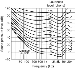
Figure 2.17 shows free-field equal-loudness contours for pure tones (observer facing source), determined by Robinson and Dadson at the National Physical Laboratory, Teddington, England, in 1956 (ISO/R226-1961). The phon scale is of equal-loudness level contours. At 1000 Hz every decibel is the equivalent loudness of a phon unit.

Figure 2.17. Equal loudness contours.

For two different sounds within a critical band (for most practical purposes, using 1⁄3 octave bands suffices) they are added in the same manner as decibel readings.(2.49)

where L^P1 and L^P2 are the individual sound levels in dB.

For example, suppose that within the same critical band we have two tones each at 70 phons. Using Eq. (2-53),

An interesting experiment in this regard is to start with two equal level signals 10 Hz apart at 1000 Hz and gradually separate them in frequency while maintaining their phon level.

They will increase in apparent loudness as they separate. This is one of the reasons a distorted system sounds louder than an undistorted system at equal power levels. One final factor worthy of storage in your own mental “read-only memory” is that in the 1000-Hz region most listeners judge a change in level of 10 dB as twice or half the loudness of the original tone.

Figure 2.18 is a chart of frequency and dynamic range for various musical instruments and the upper and lower frequency range of the average young adult.

Figure 2.18. Audible frequency range.

2.23. The Tempered Scale

The equal tempered musical scale is composed of 12 equally spaced intervals separated by a factor of

. All notes on the musical scale (excluding sharps and flats), however, are not equally spaced. This is because there are two one-half step intervals on the scale: that between E and F and that between B and C. The 12 tones, therefore, go as follow: C, C#, D, D#, E, F, F#, G, G#, A, A#, B, C (see Table 2.10).

Table 2.10. Tempered Scale

Note	Frequency ratio	Frequency Hz
C	1.000	262
C#, Db	1.059	277
D	1.122	294
D#, Eb	1.189	311
E	1.260	330
F	1.335	349
F#, Gb	1.414	370
G	1.498	392
G#, Ab	1.587	415
A	1.682	440
A#, Bb	1.782	466
B	1.888	494
C	2.000	523

2.24. Measuring Distortion

Figure 2.19 illustrates one of the ways of measuring harmonic distortion. Two main methods are employed. One uses a band rejection filter of narrow bandwidth having a rejection capability of at least 80 dB in the center of the notch. This deep notch “rejects” the fundamental of the test signal (usually a known-quality sine wave from a test audio oscillator) and permits reading the noise voltage of everything remaining in the rest of the bandpass. Unfortunately, this also includes the hum and noise, as well as the harmonic content of the equipment being tested (see Figure 2.20).

Figure 2.19. Measurement of harmonic distortion.

Figure 2.20. Methods of measuring distortion.

The second method is more useful. It uses a tunable wave analyzer. This instrument allows measurement of the amplitudes of the fundamental and each harmonic, as well as identifying the hum, the amplitude, and the noise spectrum shape (Figure 2.20). Such analyzers come in many different bandwidths, with a 1/10 octave unit allowing readings down to 1% of the fundamental (it is −45 dB at 2f ). By looking at Figure 2.20, it is easy to see that harmonic distortion appears as a spurious noise. Today, tracking filter wave analysis allows nonlinear distortion behavior to be “tracked” or measured.

2.25. The Acoustical Meaning of Harmonic Distortion

The availability of extremely wide-band amplifiers with distortions approaching the infinitesimal and the gradual engineering of a limited number of loudspeakers with distortions just under 1% at usable levels (90 dB SPL–100 dB SPL at 10–12 ft) brings up an interesting question: “How low a distortion is really needed?”

2.25.1. Calculating the Maximum Allowable Total Harmonic Distortion in an Arena Sound System

The most difficult parameter to achieve in the typical arena sound system is a sufficient signal-to-noise ratio (SNR) to ensure acceptable articulation losses for consonants in speech. It must be at least 25 dB. In that case, the total harmonic distortion should be at least 10 dB below the 25-dB SNR to avoid the addition of the two signals. If both signals were at the same level, a 3-dB increase in level would occur. Therefore (−25 dB)+(−10 dB) means that the total harmonic distortion (THD) should not exceed −35 dB.(2.50)

Therefore we could calculate

This is why carefully thought-out designs for use in heavy-duty commercial sound work have a THD of 0.8 to 0.9%:

Since the 0.8% already represents (100 2 99.2), we can write

Now, suppose an amplifier has 0.001% distortion. What sort of dynamic range does this represent?

That is a power ratio of

We can conclude that if such a figure were achievable, it would nevertheless not be useful in arena systems.

2.26. Playback Systems in Studios

Assume that a monitor loudspeaker can develop L^P=110 dB at the mixer’s ears and that in an exceptionally quiet studio we reach L^P=18 dB at 2000 Hz (NC-20). We then have(2.51)

which is equal to 92 dB. Adding 10 dB to avoid the inadvertent addition of levels gives 102 dB. The distortion now becomes

In this case, extraordinary as it is, the previously esoteric figure becomes a useful parameter.

2.26.1. Choosing an Amplifier

As pointed out earlier, the loudspeaker will establish equilibrium around 1% with its acoustic distortion. To the builder of systems, this means that extremely low distortion figures cannot be used within the system as a whole. Therefore systems-oriented amplifier designers have not attempted to extend the bandpass to extreme limits. They know that they must balance bandpass, distortion, noise, and hum against stability with all types of loads, extensions of mean time-before-failure characteristics. Most high-quality sound reinforcement amplifiers incorporate an output transformer, giving us 70 and 25 V and 4, 8, and 16 Ω outputs. In fact, connecting across the 4 and 8 Ω taps yields a 0.69-Ω output.

Example

Let the rms speech value be L^P=65 dB at 2 ft in the 1000- to 2000-Hz octave band (Figure 2.21). Let the ambient noise level be L^P=32 dB with the air conditioning on and 16 dB with the air conditioning off in the same octave band (Figure 2.22). With the air conditioning on the signal to noise ratio (SNR) is(2.52)

and with the air conditioning off

For a harmonic to be equal to −33 dB, its percentage would be

For a harmonic to be equal to −49 dB, its percentage would be

Figure 2.21. Male speech, normal level 2 ft from the microphone.

Figure 2.22. Ambient noise levels.

2.27. Decibels and Percentages

The comparison of data in decibels often needs to be expressed as percentages. The measurement of THD compares the harmonics with the fundamental. After finding out how many dB down each harmonic is compared to the fundamental, sum up all the harmonics and then compare their sum to the fundamental value. The difference is expressed as a percentage. The efficiency of a loudspeaker in converting electrical energy to acoustic energy is also expressed as a percentage. We know that

• 20 log¹⁰=20 db
• 20 log¹⁰⁰=40 db
• 20 log¹⁰⁰⁰=60 db.

Therefore a signal of −20 dB is 1/10 of the fundamental, or 100×1/10=10%. A signal of −40 dB is 1100 of the fundamental, or 100×1/100=1%. A signal of −60 dB is 11,000 of the fundamental, or 100×1/1000=0.1%. We can now turn this into an equation for finding the percentage when the level difference in decibels is known. For such ratios as voltage, SPL, and distance:(2.53)

For power ratios:(2.54)

Occasionally, we are presented with two percentages and need the decibel difference between them. For example, two loudspeakers of otherwise identical specifications have differing efficiencies: one is 0.1% efficient and the other is 25% efficient. If the same wattage is fed to both loudspeakers, what will be the difference in level between them in dB?

Since we are now talking about efficiency, we are talking about power ratios, not voltage ratios. We know that

• 10 log¹⁰=20 db
• 10 log¹⁰⁰=40 db
• 10 log¹⁰⁰⁰=60 db

and so forth.

A 0.1% efficiency is a power ratio of 1000 to 1, or −30 dB. We also know that −3 dB is 50% of a signal, so −6 dB would be 25%; (−6) – (−30)=24 dB. In other words, there would be a 24-dB difference in level between these two loudspeakers when fed by the same signal. Some consumer market loudspeakers vary this much in efficiency.

2.28. Summary

The decibel is the product of the greatest engineering minds in communications early in the last century. When it is combined with the work of Oliver Heaviside and others on impedance at the turn of the 20th century, we are equipped to handle audio levels. The concepts of dB, Z, and dBm are the tools of the professional as well as their language.

Uncited Reference

^[1]; ^[2]; ^[3]; ^[4]; ^[5]; ^[6]