Chapter 8. Interfacing and Processing

8.1. The Input

For the user, “the input” is often just a socket—often one groped for amidst a tangle of leads. This chapter untangles the details of the rarely recounted considerations that lie behind audio power amplifier input sockets that enable the signal source to connect to the amplifier (and maybe to many amps) with the least loss of fidelity and without introducing unwanted noise.

The amplifier is treated as a whole without considering the power capability or type of the output section.

8.1.1. Input Sensitivity and Gain Requirements

8.1.1.1. Definition

Input sensitivity is the signal level at the input needed to drive an amplifier up to its full capability, to just before clip, into a stated, nominal impedance, often 8 ohms. Clip may be defined as the onset of visible waveform flattening or as a certain percentage THD+N distortion factor.

An older, less used definition (favored in the 1978 IHF standard) is the signal level needed to deliver I watt into a given nominal load, say 8f2. This is fine for comparing or normalizing drive levels between amps having different power ratings, but as input sensitivity per se has no particular merit, the usefulness, for real amplifiers and speakers of widely varying power capabilities and sensitivities, ends there.

8.1.1.2. Description

Sensitivity is usually expressed as a voltage, either directly in volts or millivolts (1/1000ths of a volt), or in dBu. Mostly, sensitivity figures are assumed to be rms values (cf. peak) and also specified with a steady sine wave, and for power amps in particular, with loading—all unless stated otherwise. If a peak (or any other non-rms) voltage value is cited, the maximum output to which it is referred must also be cited likewise, so like is being compared with like.

8.1.1.3. Variables

The sensitivity of an amplifier depends (as defined earlier) on gain and swing. If an amp’s output power rating, hence voltage swing capability into a given load impedance, were increased, maintaining the sensitivity requires more gain from the amplifier. This is a consideration for the maker and the installer who uses different sizes of a given design.

8.1.1.4. Do-It-Yourself Gain Resetting

For those uses with two or more different models and/or makes of amplifier, it is likely that sensitivities (however referred) will differ. Gain controls may not be present or it may be desired not to use them. If so, to align the system (ideally within a fraction of a dB), all the amps enter clip at about the same drive level and the gain(s) of one type of amp will need changing. Usually, any gain controls are assumed to be at maximum. Then any “accidental adjustments” can only cause reduced, not excess, gain.

In most well-designed, conventional high NFB power amps, gain may be changed up or down easily by changing one (global feedback) resistor per channel. The part being changed is usually in the output section. Changing gain by up to +10 dB or down by as much as –6 dB should have relatively little effect on sonic quality, assuming that RF stability is not upset. However, noise will be altered pro-rata.

In low- and zero-feedback designs, the availability of gain changing is far less, and the effect on both measured and sonic performances of even a modest 10-dB (×3) adjustment will be far more marked.

8.1.1.5. Gain Restriction

In some power amp designs, gain changes may be unavailable because they would upset RF stability, imperil a finally balanced gain/feedback structure, or violate some arbitrary %THD+N limit or other basic performance indication. Thus amplifiers from a product family spanning a range of output power ratings may have very similar gains (+ to –3 dB); thus sensitivities (mV, V) almost commensurate with their ascending voltage swing. The upshot of this approach is (for example) a 2-kW 8fΩ amplifier, which only provides 100 W at normal drive levels (0 dBu say). The +13-dBu/3.5-V rms input drive needed for full output makes it safer and more likely that the high swing will be kept in reserve as an inviolate headroom.

In other words, in lieu of increased gain when output swing is increased, such an amplifier will need to be driven harder, that is, rated less sensitive. If the headroom achieved is ever used, then the higher input drive levels can cause increased distortion in the input stage. This effect will be noted most in esoteric amps with low feedback, but is still there in conventional high NFB amps.

8.1.1.6. Gain and Fidelity

As noted, the positive side of having high swing amplifiers desensitized, by not increasing gain commensurate with the increased voltage swing is that headroom occurs by default if the system’s level/gain settings are not then altered. Reduced gain also reduces the risk of speaker damage by accidental loud blasts, dropped mics, styli, etc. Also, the audibility of the system’s residual noise is lowered.

8.1.1.7. CM Stress

In conventional power amplifiers with high NFB, “common mode distortion,” measurable as %THD+N,^[1] occurs because of common-mode voltage stress on the input stage, whether differential or single ended, with the latter suffering CM stress if, as is common, it is noninverting. The threshold voltage, ‘Vth’—above which the input voltage to such an op-amp-type input becomes highly nonlinear when open loop may be sonically significant.^[2,3] These setbacks may not be revealed with conventional tests, notably %THD+N, which can contrarily show lowered distortion at high input drive test levels, because the noise (+N) may “out-reduce” the rising common mode distortion.^[1]

8.1.1.8. Real Figures

The sensitivity of every amplifier needs to match the zero (normal) levels of sources it is intended to be driven by. These vary. The upshot of all the factors is a spread of amplifier sensitivities that users know all too well (Table 8.1).

Table 8.1. Range of Input Sensitivities

Category	In volts	In dBu
Home hi-fi	30 mV to 2 V	–28 to+8
Home studios	100 mV to l V	18 to+2
Pro-audio	775 mV to 5 V	0 to+16

Ideally, there could be just one input sensitivity for all these uses. One that most could accept is the de facto professional standard of 0-dBu alias 775 mV. As a general rule, most lightweight domestic hi-fi and home studio equipment is likely to be more sensitive than 0 dBu, with pro equipment likewise less sensitive.

However, as just discussed, a specific lower value, as low as 30 mV, may be best (at least in high NFB circuits) from the viewpoint of circuit and device physics for absolute best linearity.^[2] However, the higher voltages that are mostly needed by desensitized high swing amplifiers (e.g., driving 2 V or +SdBu and above to clip) confer the highest SNR, hence dynamic range, and also the highest RF EMI and CMV immunity. So the best of both these worlds appears not to be immediately reconcilable.

As most amplifiers are not pure voltage sources, when driven with continuous, high-level test signals into a real (or simulated) loudspeaker load (as opposed to an ideal, simple resistive load), the sensitivity (for a given clip level) can appear to increase at some frequencies, as the maximum output voltage with a conventional amplifier having an unregulated supply is reduced by typically by –0.5 to –2 dB. The average shortfall is likely to be less with program, at least at mid- and high frequencies. It follows that there is a complex frequency-conscious and dynamic peak-to-mean disparity in practical amplifiers’ sensitivity ratings. The purer the voltage source, the less this can happen.

8.1.1.9. Gain and Swing

Table 8.2 shows the gain requirements both in dB for some “round-figured” voltage swings, and how the nominal power then varies into 4 and 8 ohms.

Table 8.2. Power Amp Gains for 0-dBu Sensitivity @ Clip ⇒ Means ‘Into’

Gain (dB)		rms voltage swing (V)	Average power ⇒ nom 8 Ω (W)	Average power ⇒ nom 4 Ω (W)
+24	=×16	12.5	19	38
+30	=×32	25	78	156
+33.5	=×48	37.5	176	352
+36	=×65	50	312	624
+40	=×97	75	703	1406
+42	=×129	100	1250	2500
+44	=×l61	125	1953	3906

For other sensitivities, gains are determined easily by appropriate subtraction or addition, for example, for +4 dBu, subtract 4 dB from the indicated gain(s) and for –10 dBu, add 10 dB to the indicated gain(s).

8.1.2. Input Impedance (Zⁱⁿ)

8.1.2.1. Introduction

The amplifier’s input impedance is the loading presented by the amplifier to the signal source driving (or “looking up” or “into”) it.

Impedances (often abbreviated ‘z’) are rated in ohms (Ω). As in this case, ohmic values are nearly always over 1000; the counting is usually in thousands (k). 10 k or 10 kΩ (“10 k ohm”) is easier to say than “ten thousand ohms.” When near a million or over, ‘M’ for ‘Mega’ is used, for example, 1 MΩ is 1000 kΩ.

8.1.2.2. Common Values

With ordinary, high NFB power amplifiers, high input impedances (high Zⁱⁿ, say above 10 kΩ), to 1 MΩ or more, are readily attained. For most sources, this is analogous to very light loading. However, in most cases, power amp input impedances are commonly at the low end of this range, at between 10 and 22 kΩ. This restricts noise and buzzes when (particularly unbalanced) inputs are left open, unused, or floating, especially when cables are unplugged at the source end. This is less of a problem with short cables and in domestic environments.

The nominal values of amplifier input impedances vary widely. As a rule, professional equipment is defined in Table 8.3.

Table 8.3. Power Amplifier Input Impedances

Type of power amplifier	Zin range
Domestic, seperated. and integrated	10 k–200 kΩ
High-end domestic, esoteric	600–2 MΩ
Professional	5 k–20 kΩ
Vintage professional	600 Ω

If balanced, Zⁱⁿ is the differential mode Z.

The input impedance of equipment may be described as the source’s load impedance. This is true enough at frequencies below l kHz. However, load impedance (since the signal source may be across a room, 100 yards down a hall, or even half-way across a field) is the totality of loading, namely including all the cable capacitance, which takes effect increasingly above 3 kHz.

8.1.2.3. Audio is Not RF

Precise “impedance matching,” where specific impedances (often 50 or 75 ohms) must be adhered to, is correct for radio frequencies, where cables above a meter or so act as a transmission line.^[4] But at the highest audible frequencies (20 kHz) even a 200-m-long input cable in a stadium PA system doesn’t behave as a transmission line.

Where the wavelength (the dual of frequency) is a fair fraction, say 20 or 10 times greater than the cable, cables look mainly like the respective sums of their resistance, capacitance, and inductance. As the ratio falls, the cable begins to behave increasingly like a transmission line.

8.1.2.4. Voltage Matching

Since the widespread use of NFB (50 years ago), the majority of power amplifiers’ inputs have been voltage matched. This means that the source impedance is low—much lower (at least 10 times less) than the total destination, or load impedance.^[5,6] The intention is to transfer the signal, which is encoded as a voltage “wiggle,” without significant loss of headroom, dynamic range, or detailing.

The source’s impedance—whatever’s feeding the amplifier(s)—also has to be low enough and remain so at hf to support a fiat hf response into the capacitative loading of likely cable lengths. Voltage matching is defined by de facto industry practice, in the IEC.268 standard. Here, recommended input impedances are 10 kΩ or over and equipment source impedances are 50 Ω or less. This is easily memorized as

Looking back from amp:	Looking up from amp:
≤50Ω⇐	⇒≥10kΩ

With voltage matching there is no sharply defined “right” impedance. Except that in high common mode rejection (CMR) balanced systems and high resolution stereo systems alike, an amplifier’s individual input impedances may be ultra-matched. Since with voltage matched systems, the wanted input signal is a voltage, the ideal, “noninvasive” amplifier input or load impedance would appear to be very high, say 1 MΩ. Then only minuscule current would be taken from the source.

8.1.2.5. High Impedances

Some high-end hi-fi makers have taken the high impedance route, claiming better sonics. This may be inseparable from the circuitry used to create the high-Z conditions, and not necessarily down to the high-Z conditions per se.

In power amps with low (or zero) feedback, and using bipolar junction transistors (BJTs) in the input section, high input impedances (above 10 kΩ) can be more difficult to implement consistently. On this basis, the early transistor amplifiers sometimes had their inputs rated in μA of input current drawn! In contrast, there is usually no difficulty attaining impedances as high as 1 MΩ or more, when the input stage parts are valves, JFET or insulated gate FET (MOSFET) or any combination of these—whether loop or local feedback is zero, low, or high.

When unterminated, such high impedance circuits are noisier (hissier) and far more liable to allow parts to be microphonic than lower (“normal”) impedance ones.^[7] Demonstration is simple enough: try tapping the appropriate capacitors with an insulated tool while listening with full-range speaker(s) connected. High impedance inputs can also be the cause of difficulties and compromises with direct coupling. However, unless the input is direct coupled, or is at least coupled via very large capacitors, LF and subsonic microphony and electrostatic noise pick-up will not “see” the lower source impedance and will persist in accordance with the high impedance.

8.1.2.6. Low Impedances

As input impedance is lowered, there is less microphony and electrostatic noise pick-up when the amplifier inputs are disconnected, even with unshielded cabling. However, loading is increased, as is ultimately the susceptibility to magnetic field noise pick-up, which is much, much harder to shield against.

8.1.2.7. Loading

A single load of (say) l kfΩ may or may not compromise the source’s performance. But two or a few of such loads almost certainly will, unless the source is rated appropriately (see later). Low impedance inputs are also the most easily damaged if one amp’s output is accidentally connected to another’s input. Added protection would add complexity, increase the cost, and likely degrade sonics.

8.1.2.8. In Tandem

In professional (and even a few domestic) applications it is normal for each signal source to drive more than one amplifier input. The loading of amplifiers driven in tandem is cumulative: each added amplifier reduces the impedance (or increases the loading) pro-rata in accordance with its impedance. Assuming conventional power amplifiers with 10 kf2 input impedance, the reciprocal pattern is shown in Table 8.4.

Table 8.4. The reciprocal pattern of conventional power amplifliers (with 10 kΩ input impedance)

No. of amps in tandem	Total Zin
×l	10kΩ
×2	5kΩ
×3	3.3kΩ
×4	2.5kΩ
×5	2kΩ
×6	1.7kΩ
×l0	1kΩ
×15	666kΩ
×20	500kΩ

Note that there are very few types and models of the likely sources (e.g., active crossovers, delay lines, preamps) that are rated and able to drive impedances of below 600 ohms without degraded performance. Much pro-gear is rated and even specified for 600 ohms, but still gives its best measured and sonic performance into 2 k or even higher.

For large tandem systems, existing equipment usually has to be retro-fitted with special line-driver amplifiers, or these are added as independent units, in line. Line drivers used in live sound practice do not expand the allowable loading by much, usually down to 300 ohms and possibly as low as 75 ohms. To be sure, only 50% of this rating would be used. The rest allows for tolerances, variables (see later), add ons, and the cable’s capacitance loading at hf. In a major concert where 100 or more power amps have been required to handle just one frequency band alone,^[8] the signal was split among up to 10 line drivers, all daisy chained off 1 line driver. This method is far preferable to having multiple crossovers, which might superficially simplify the signal path, but would also introduce near impossible set-up and band-matching demands.

8.1.2.9. Multiconnection

When one signal has to feed many amplifiers, it is normal to connect the amplifiers by daisy chaining. To permit this, amplifiers made for professional use have both female (input) and also male (output) XLR (or other, gendered or ungendered in/out) connectors, linked together in parallel. “Daisy chaining” means physically, as the name suggests, that a short cable “tail” carrying the input signal loops from one amplifier to the next in the rack or array. The signal being passed on is not really entering each amplifiers’ input stage, but merely using the input sockets and case-work as a durable and shielded Y-splitting node. An alternative would be to make up a hydra-headed cable, that is, one splitting into n separate feeds. This would take up far more space and is far less flexible, but might prove the next best method if amplifiers without input “link-out” sockets have to be used.

8.1.2.10. Ramifications

Professional power amplifiers, which are the sort most likely to have long cables connected to their inputs and to reside in electrically noisy environments, mainly eschew impedances much above 10 k. However, if they’re to be usable for live sound, their makers also can’t welcome any much lower impedance, as this would further limit the number of channels that can be daisy chained off a given line driver. In most multi-amp setups, the source that is being loaded is usually one of the band outputs of an active crossover, rated for 600 ohms with the NE5534 or 5532, 1977 IC technology that remains a de facto standard. In this common case, depending on the allowance for cable capacitance, between 10 and 15 amplifier channels (at most) should be driven.

8.1.2.11. Variables

As with other electronic equipment, input impedance is a function of electronic parts whose behavior almost inevitably varies with frequency and almost always depends on temperature. With unbalanced inputs, input impedance will also usually vary somewhat with the setting of the gain control (attenuator), if fitted.

Figure 8.1 shows how the input impedance of a typical, minimal power amplifier with an unbalanced input (Figure 8.2) varies across the frequency range. A 10kΩ gain control is assumed and is here backed off just ldB. Note how the impedance in most of the audio band is almost constant at the scale used. Then notice how the impedance drops off (so the loading increases) at high audio frequencies, and more so at higher radio frequencies (Y). At low frequencies, if anything, the load impedance increases (X).

Figure 8.1. Input impedance (load) variation in a typical, simple unbalanced power amplifier input stage.

Figure 8.2. A typical unbalanced input stage.

Figure 8.3 shows how the same input stage’s impedance varies (without changing anything else) as temperature is changed from 15° to 85°. In other words, what can happen to the input impedance when an amplifier is “cooked?” For the most part, impedance increases, which will do no harm. However, in live work it might just alter a howl round threshold, as the higher load impedance allows the signal voltage to rise ever so slightly.

Figure 8.3. Impedance variation in a typical unbalanced power amplifier input stage as the amplifier warms up.

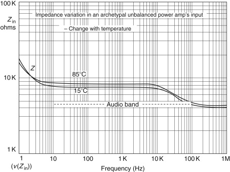
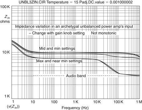
Figure 8.4 shows how the input impedance typically varies as the gain is adjusted. Because the change with each 30° rotation step is nonmonotonic, Zⁱⁿ goes up and then comes down, as you might expect. A 10kΩ log pot is assumed.

Figure 8.4. Impedance variation in a typical unbalanced power amplifier’s input stage as the gain control is swept.

Ideally, an amp’s input impedance would remain constant despite these changes. In unbalanced circuits, there is not much harm as long as any change in impedance is gradual and stays above certain limits, and anything that isn’t like this happens well above (or even further below) the audio band. Staying constant is far more important in balanced circuits.

8.2. Radio Frequency Filtration

8.2.1. Introduction

Music starts out as air vibrations. These are not directly affected by electromagnetic (EM) waves, except while they are passing through an audio system in the form of electronic signals. Planet Earth has long had natural EMI, in the form of various electric and magnetic storms; both those occurring in the atmosphere and those occurring on the “surface” of the Sun and Jupiter in particular. Since 1900, the planet has increasingly abounded in human-made EMl babble, comprising electromagnetic energy fields and waves, some continuous, some pulsed, and others random. As stray signals nearly always have nothing to add to the music at hand, and most are profoundly unmusical, and as EMI permeates almost everywhere above ground unless guarded against, music signals require “pro-active” protection.

EM waves used for radio broadcasting and communications mainly start in earnest at 150 kHz (in the United Kingdom and continental Europe) and above, and continue to frequencies l0,000 times higher. However, special radio transmissions (for submerged submarines, national clocks, and caving) may use frequencies below 100 kHz and even those below 20 kHz.

8.2.2. Requirement

All active devices are potentially susceptible to EMI. BJTs, all kinds of field effect transistors (FETs), and also valves can all act as rectifiers at RF, demodulating radio transmissions. However, this is very much more likely with BJTs, as the nonlinearity of a BJT’s forward biased base-emitter junction that gives rise to rectification is triggered by considerably lower levels of RF voltage or field strength. All kinds of FETs and valves are relatively “RF proof” in comparison. Oxidized copper, generally dirty contacts, crystalline soldered joints, or wrong metal-to-metal interfaces can all act as RF detectors as well, through rectification.

8.3. Balanced Input

Balanced inputs, when used properly, can clean up hums, buzzes, RFI, and general extraneous rubbish. When not used properly, the balanced-input’s object may be partly defeated, but the connection will probably still improve the amplifier’s and system’s effective SNR.

8.3.1. Definition

To be truly balanced, a balanced input and the line coming in and the sending device must all have equal impedances to (signal) ground, to earth, and to everywhere else. Also, the signal must be exactly opposite in polarity but equal in magnitude, on each conductor.

8.3.2. Real Conditions

In practice, the signal is not of exactly opposite polarity. At high frequencies (and low frequencies in some poorly designed equipment), phase shifts add or subtract up to 90° or more, from the ideal 180° polarity difference. Otherwise the requirement for having a signal of opposite sign on each conductor is usually met. The exception is when one-half of a ground-referred, balanced source has been shorted to ground. Not surprisingly, this degrades the benefits of balancing.

8.3.3. Balancing Requirements

8.3.3.1. Input Impedances

The norm in modem pro-audio equipment is 10 kΩ across the line. This is commonly known as a “bridging load.” It is also the differential input impedance.

The common mode impedance, what any unwanted, induced noise signals will see, is often (but not always) half of this, for example, 5 kΩ in this case.

Considering the hum/RF noise rejection capability of an effective balanced input, input impedances much higher than 10 kΩ, say, 500 Ω, would seem feasible and useful in professional systems. However, if the input resistance is developed by the ubiquitous input bias path resistors connected from each input to the 0-V rail, then there are limits to the usable resistance, before the input stage’s output offset voltage becomes unacceptably high. Although low V^oos op-amps exist, a number of otherwise good ICs for audio have execrable DC characteristics, as IC designers do not appear to comprehend that good DC performance is a most helpful feature for high performance audio. In this case, input impedances above 15 to 100 kΩ are found to be impractical, depending on bias current.

A galvanically floating input (i.e., the primary of a suitably wired transformer) has no connection to signal 0 V (as it has no bias currents), so there can be a very high common-mode impedance, say, l M or more, up to modest RF. This aids rejection.

Conversely, differential impedances of less than l Ok increase the influence of such random, external factors as mismatched cable core-to-shield capacitances.

8.3.4. Introducing Common Mode Rejection

Common mode rejection is an equipment and system specification that describes how well unwanted common mode signals, mainly hum and RF interference, are counteracted when using balanced connections.

8.3.4.1. Minimum Requirements

At the very least, all the equipment in a system must have a balanced input (alias a “differential receiver”). CMR can be improved and made more rugged when balanced inputs are used in conjunction with balanced outputs (alias “differential transmitters”), but this is not essential.

8.3.4.2. What Does CMR Achieve?

Common mode rejection action prevents the egress and build-up of extraneous hum, buzzes, and RFI when analogue signals are conveyed down cables, and between equipment powered from different locations—all the more so in big or complex systems. CMR helps make shielding more effective by canceling the attenuative residue, the bit that any practical shield “lets through.”

Sending the signal on a pair of twisted and parallel conductors ensures that this latter residue and any other stray signals that are picked up en route are literally coincident and appear “common mode,” that is, equal to each other in size and polarity. A tight enough twist makes the conductors almost experience interfering fields as if they occupied the same space. This is true below high RF (200 MHz, say), when averaged out over a cable’s length.

In contrast, the wanted, applied signal from both balanced and unbalanced output sockets is distinguished while being no less equal in size by appearing opposite in polarity on each input “leg,” called hot and cold.

CMR also makes shielding more effective by freeing it from signal conveyance, enabling it to be connected at one end only, according solely to the dictates of optimum RF suppression and/or individual system practice. Breaking the shields through connection also prevents (or at least lessens) the build-up of the mesh of earth loops that causes most intractable hums and buzzes. CMR is also able to cancel differences between disparate, physically distant and electrically noisy ground points in a system.

Above 20 kHz, even a modest CMR lessens the immediacy of the need for aggressive RF filtering. RF filtering can take place at higher frequencies, and both the explicit and the component-level effects on the audio may be diminished accordingly.

Figure 8.5 shows the CMV that CMR helps the audio system ignore. Even when connection to mains safety earth is avoided by ground lifting (ground lift switch open) or by total isolation (switch open and ground lift R omitted), considerable capacitance frequently remains, through power transformers and wiring dress.

Figure 8.5. Most of the common mode noise that CMR defends against is either RF and 50/60 Hz fundamental intercepted in cabling (Vcml) or 50/60 Hz hum+harmonics caused by magnetic loop, eddy, and leakage currents flowing in the safety ground wiring between any two equipment locations (Vcm2).

Overall, the rejection achieved (which is a ratio, not an absolute amount) is described in minus (–) dB. Often the minus is understood and omitted. In plain English, “CMR=40 dB” means “all extraneous garbage entering this box will be made 100 times smaller.”

8.3.4.3. What CMR Cannot Do

Like the stable door, the one thing CMR can’t do is remove unwanted noises that are already embedded in with the music. It follows that just one piece of equipment with poor CMR, and in the wrong place, can determine the hum and RFI level in a complex studio or PA path.

The ingress of common mode noise, called mode conversion, is cumulative, as each unit in the chain lets some of it leak through. As a result, the CMR performance and/or interconnection standards of all the equipment in complex systems (e.g., multiroom studios and major live sets) must be doubly good.

The higher CMR of well-engineered equipment (80 dB or more) provides a safety factor of 100- to over 1000-fold over the minimum 40 dB that is common in more “cheerful” products. However, the higher CMRs are more likely to vary with temperature and aging, as with all finely tuned artifacts.

8.3.4.4. Relativity Rules

The size of common mode (noise) signals is not fixed or even very predictable; they may range from microvolts to tens of volts. CMR is just a layer of protection. Forty dB of protection is not much against 10 V of CMR, but it is definitely enough for 1 μV.

8.3.4.5. Sonic Effects of RF

Radio frequency interference is a common mode noise, and sources of RF go on increasing. In a competently wired system in premises away from radio transmitters and urban/ industrial electrical hash, a modest rejection no better than 40 dB has previously seemed good enough to make inaudible induced 50/60-Hz hum and harmonics, and the “glazey” sound of RFI and RF intermodulation artifacts. Unfortunately, RFI artifacts aren’t always blatant, and when any sound system is in use, they’re the last thing that users are likely to be listening for the symptoms of. However, even if there are no blatant noises, inadequate CMR can allow ambient electrical hash to cover up ambient and reverberative detail.

8.3.4.6. System Reality

The CMRs discussed are those cited for power amplifier input stages. The actual system CMR is inevitably cumulatively degraded by the cabling and the source CMRs. However, it can be maintained by ensuring all three have individually high CMRs and have highly balanced leg impedances. Lines driven from unbalanced sources give numerically inferior results, but often quite adequate ones (subject to appropriate grounding and cable connections) in low-EMI domestic hi-fi and studio conditions, where equipment connections are also compact, and even in outdoor PA systems, in an open countryside.

8.3.4.7. Summary

Generally, 20 dB is a low, poor CMR, 40 to 70 dB is average to good, and 80 to 120 dB or more is very good and far harder to achieve in a real system. In a world where some audio measurements have had their credibility undermined, it’s reassuring to know that with CMR, more dBs remain simply better.

8.4. Subsonic Protection and High-Pass Filtering

8.4.1. Rationale

All loudspeakers have a low-end limit; their bass response does not go endlessly deeper.

Subsonic (infrasonic) information, comprising both music content and ambient information, may occur below the high-pass “turnover” frequency (or low-end roll off) of the bass loudspeaker(s). It will not be reproduced efficiently.

Note: While potentially within humans’ aural perceptive range, subsonic signals are “below hearing” (strictly infrasonic) in the sense of being “out-of-band” to, and only faintly or at least reducingly reproducible by, the sound system.

Loudspeakers vary in their ability to handle large subsonic signals. Small ones may or may not be heard but won’t ever cause damage. Large subsonic signals are more risky with some kinds of loading. An approximate ranking of subsonic signal handling robustness is shown in Table 8.5. Individual designs can vary widely, however.

Table 8.5. Loudspeaker Subsonic Handling (Infrasonic Handling)

More robust ⇑	Transmission lines
	Differentially loaded cabsa
	Properly arrayed bass horns
	Sealed boxes
	Open-backed cabs
	Large cone-vented enclosures
Less robust ⇓	Small cone-vented enclosures

^a Alias band pass or push–pull.

8.4.2. Subsonic Stresses

Other than straining the speaker(s), if the amplitude of the subsonic (really infrasonic) signal(s) is large enough, then significant amplifier capability will be wasted. At the very least, the unrealizable portion will cause unnecessary amplifier heating and electricity consumption.

If the amplifier is also being driven hard, the presence of a large subsonic signal will reduce the threshold for clipping and also thermal shutdown. The amplifier will behave as if rated at only a fraction of its actual power capability. There are broadly two approaches to the problem.

8.4.3. The Pro Approach

Subsonic filtering may be regarded as an essential part of editing and sweetening in recording. “Subsonic” frequencies (“sub” here being rather loosely designated as any “out of context/too-low bass information”) are usually removed before amplification by HP filters (HPF) with fixed, switchable, or sweepable roll-off frequencies, usually available on each channel or group of a mixing console. Alternatively, HP filtering may even be available “up front” as a switch on some microphones or on portable, location tape machines.

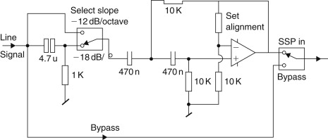
Generally, such filters are at least –12 dB/octave and, more usefully, the steeper –18-dB/octave (Figure 8.6) or even –24-dB/octave. They may be occasionally appended to professional power amplifiers, as well as to preceding active crossovers, on the basis of providing “maximum” (read: brute force) protection at all costs, in this guise they are described as “subsonic protection” (SSP). Often this facility is superfluous and repeated needlessly, as the mixer and active crossover already do or can provide subsonic filtering.

Figure 8.6. Typical high-pass (subsonic protection) filter circuitry.

8.4.4. Logistics

The mixer can provide SSP most flexibly per channel, solely for those sources requiring filtration. The active crossover may provide overall back-up subsonic protection, in case a mic without HPF’ing on its channel is dropped.

When subsonic protection is fitted to and relied upon in amplifiers alone, there will be an enforced and unnecessary repetition and diversification of resources in any more than the simplest, two-channel PA. If subsonic filter provision is made in an amplifier, it should be switchable (or programmable or otherwise controllable) so that its action can be removed positively when not required.

8.4.5. Indication

A few power amplifiers have light-emitting diodes (LEDs) (often jointly error indicators) that indicate subsonic activity or protection shutdown arising from excess subsonic levels. This kind of protection is most common where the maker is also a speaker maker or where the amplifier is closely associated with a particular speaker, as the protection’s frequency–amplitude envelope that will allow the most low frequency action is very specific to the cabinet and driver used.

Overall, in high performance professional power amplifier designs benefiting from modem knowledge, filtration and any HP filtering are avoided as far as possible or else minimized by adaptive circuitry.^[9]

8.4.6. Hi-End Approach

In “hi-end” hi-fi and professional power amplifiers, high-pass filtering is (or should be) depreciated or at least kept to the bare minimum, for two reasons.

First, all practical HP filters progressively delay low frequencies relative to the rest of the music. Every added HP filter pole only adds to this “signal smearing.”^[10] Simulation in time and frequency domains shows this.^[11]

Second, HP filters require the use of capacitors. Capacitors that are almost ideal for audio and not outrageously expensive and bulky are limited in type and values. Capacitors that are faradically large enough not to cause substantial “signal smearing” are, in practice, medium-type electrolytics, and not in practice nor in theory anywhere near so optimal for audio as other dielectric types.

For these reasons, even routine HP filtering (alias DC blocking or ac coupling) may be absent altogether. Figure 8.7 shows the points where HP filtering occurs in the majority of otherwise direct- and near-direct-coupled power amplifiers.

Figure 8.7. High-pass filter capacitor positions. The potential locations of DC blocking/HPF capacitors in the signal path of conventional transistor power amplifiers, assuming that gain blocks (the triangles) are internally direct coupled.

8.4.7. Low Approach

In “consumer-grade” audio power amplifiers, HP capacitors are made as small as possible in value while maintaining what is judged by casual listening or first-order theory to be an acceptable point for the bass response low cutoff frequency (f3^L). The result is considerable HP filtering, permanently engaged. Subsonic signals may then rarely pose a problem, but sonic quality may be degraded up into midfrequencies, while a great deal of the music’s ambient cues is lost.

8.4.8. Direct Coupling

When all HP filtering is removed, a power amplifier becomes direct—or ‘DC’ (direct current)—coupled. ‘DCC’ would have been better, but that now means something else. Extending the response to zero frequency, that is, “down to DC,” is achieved readily at the design stage with most transistor topologies. The advantages are sonic, and substantial, due to the excision of intrinsically imperfect parts and the removal of an intrinsically unnatural filtration, and the signal-delay and the possible charge accumulation on asymmetric music signals it brings. For this is the truth of all signal path HPF capacitors, both those in series and in NFB arms. Whether DC coupling is safe or workable in a particular amplifier is a separate design question.

With conventional valve amp topologies, the response to DC is not fully achievable, except in the few workable ‘OTL’ designs. However, it is still possible to direct couple the remainder of a valve amplifier, with global DC NFB taken before the transformer. In fact, the first precision DC amplifiers were valve op-amps.

8.4.8.1. Direct Current Management

With direct-coupled circuitry, unwanted DC “offset voltages” will be amplified by the power amplifier’s respective stage gains. Excess DC is of great concern and must be avoided. It can be (i) produced internally, by mismatches in resistor or semiconductor values or by intrinsic topological asymmetry or (ii) introduced externally, from preceding DC-coupled signal sources.

Internally produced DC offsets may be kept to safe levels by precision in design and component selection. This requires matching of two or three apposite parameters of the differential pair at the front end of each stage, assuming some version of the conventional high NFB “op-amp” type of architecture. The “pair” might be BJTs, FETs, or valves. And to ensure that the source resistances (at DC) seen by each input leg are the same, or close, and not too high either, depending on bias current. If the resistor values then conflict with CMR, the latter should have priority, in view of EMC requirements, and the nonrecoverability of the CMR opportunity. Direct current balance may be restored by other means, for example, current injection.

Externally applied DC, appearing on the inputs, because of essentially healthy but imperfect preceding equipment, will usually be in the range of 0.1 to 100 mV. More than +/–100 mV would suggest a DC fault in the preceding source equipment. Assuming a gain of 30×, this would result in 3 V at the amplifier’s output. Because such a steady offset will eat up headroom on one-half of the signal swing, the clip level is lowered asymmetrically. A direct coupled power amplifier should not be harmed by this and should also protect the speakers it is driving, but equally it is entitled to shut down to draw attention to such an unsatisfactory situation. In the most advanced designs of analogue path yet published,^[9] DC coupling is adaptive: if DC above a problem level persists at the input, DC blocking capacitors are automatically installed and the user is informed by LED.

Some low-budget domestic power amplifiers have long offered part and manual direct coupling. The power stage may not be wholly direct coupled, but at least the DC blocking capacitor(s) at the input can be bypassed via a second “direct” or “laboratory” input. The user is expected to try this but revert to the ordinary ac-coupled inputs if DC on the source signal is enough to cause zits and plops. A blocking capacitor(s) at the input can be bypassed via a second “direct” or “laboratory” input.

8.4.8.2. Autonulling

Direct current offset may be continually forced to near zero volts by a servo, which is another name for brute-force VLF and DC feedback, applied around an amplifier overall, or just the input or output stage. Servos have been de rigueur in U.S. and U.S.-influenced high-end domestic power amplifiers for some years. Alas, those who have designed them into high-performance power amplifiers have clearly not thought through the consequences. Tellingly, servos are not usually nor likely to be found in amplifiers with truly accurate sounding bass.

The reasons are clear enough today: servos cause the same or even wilder distortions in LF frequency and/or phase response, and/or signal delay vs. frequency (group delay). Figure 8.8 shows this.

Figure 8.8. Direct current servo circuits cause at the very least the same phase and delay error as using a DC-blocking capacitor conventionally. The upper graph shows the frequency response of a standard two pole servo (2×{1 M.O×470 nF}). The lower graph shows the phase shift, which is clearly nonlinear below 85 Hz—place a ruler against the line. The curvature indicates a frequency-dependent signal delay, hence smearing (after Deane Jensen). An alternative, custom three-pole compensating type (C3P) is plotted. This overcomes the smearing, as the phase shift is much less than 0.1º above 5 Hz, but the amplitude (upper) is now peaking below 1 Hz.

They also compromise the integrity of the circuitry they are wrapped around by increasing noise susceptibility, while the capacitor imperfections that DC coupling is supposed to overcome are reintroduced, as distortion-free DC servo action depends on an expensive, bulky, high-performance capacitor for integration. In this way, the DC servo returns us to before square one, with the added cost and complexity. Worse, the original thinking behind servo’ing was to save money (!) on input transistor and part matching, as a servo will “fix” any DC in its range, often up to +/–5 V, including DC appearing on the equipment input. This is neat, but like so many “smart” options, DC servo’ing is not quite suitable for audio.

8.5. Damage Protection

The input stages of most audio equipment are unprotected. This approach appears to save on parts cost, complexity, and sonic degradation; however, in reality, it may indeed cause costs and degraded sonics. The inputs of power amplifiers are certainly among those most likely to sustain input voltages that may be damaging to the active parts inside.

8.5.1. Causes

Typical culprits include first, large signals from line level sources, and from amplifier outputs, experienced through accidental connections (see Section 8.5.2). Here, excessive signal voltages that could be applied could range from a few volts, up to 230 V rms, and from below 10 Hz to above 30 kHz.

Second, the outputs of crossovers or consoles, or misconnected amps, which are kaput and have DC faults, so the output voltage might range from +/–10 V to up to +/–30 V for line sources, and up to +/–160 V DC for power amplifiers, but more typically +/–30 to +/–90 V DC.

8.5.2. Scope

The parts most at risk from excess input voltages are the solid-state active devices, particularly discrete BJTs, and most monolithic IC op-amp input stages.

Valves are relatively immune to input voltage abuse. They are most likely to be harmed by gross overdrive conditions that bias the grid positive so a damagingly high current flows.

J-FETs and MOSFETs are next most rugged. MOSFETs are most susceptible to gate-source overvoltage, but gate-source protection is straightforward and effective.

IC input stages are the most fragile. Due to IC structure, even FETs, when monolithic, may have parasitic weak points. For long-term reliability, currents flowing into or out of IC op-amp pins^[12] must always be kept below 5 mA.

8.5.3. Harmful Conditions

There are two kinds of potentially damaging input voltages: (1) common mode and (2) differential mode. Either may occur when a power amplifier is in (i) the on state or (ii) the off state, giving four possibilities.

8.5.4. On-State Risks

When an amplifier employing BJTs at the front of its input stage is on, powered up, and settled down, it can sustain relatively high differential (signal) voltages without damage. Generally, in high NFB op-amp and other dual-rail based designs, the max differential voltage is a volt below the supply rails, hence a maximum differential voltage ranges from +/–14 V for input stages working from +/–15-V supplies, up to +/–30 V or even over +/–100 V, where the input stage transistors operate from the same or else similarly high supplies, as the output stage.

Long before differential overload, the input stage will be driven strongly into clip. Provided the amplifier has clean recovery, an overvoltaging may pass unnoticed if the high differential voltage only lasts I mS. Yet this is plenty long enough to damage a semiconductor junction. In BJTs, the most vulnerable junction is the base emitter, when reverse biased.

Under the same powered-up conditions, common-mode voltages above +/–10 V can damage unprotected BJT input stages. In large systems, the common-mode voltage can be this high, commonly comprising 50/60-Hz AC and harmonics, and arising from differences in grounding or AC power potentials.

The input stage’s supply rail voltage usually has a large bearing on the maximum safe DM and CM input voltages. Here, low supply voltages may do no favors.

8.5.5. Off-State Vulnerability

When an amplifier using BJTs is switched off, both differential and common-mode voltages as low as +/–0.5 V may be damaging. Users are advised to always power-up preceding equipment before the power amps. This is universal practice among informed users, both domestic and professional. However, if the prepowering of the source involves the passage of signals above 0.Sv peak to amplifier inputs, then unless the transistors behind the sockets are protected before the amp is powered-up, they may well be damaged. This mode of subtle, progressive damage and sonic degradation to analogue electronics has yet to be widely recognized. It can be overcome without changing otherwise sensible practices, by suitably designed input protection.

8.5.6. Occurrence Modes

Damage to input devices may be catastrophic if the overvoltage causes high currents to flow. This is rare.

Otherwise, with BJT inputs, damage may be subtle. Transistor parameters are degraded but NFB action initially hides the worst. Telltale signs would be changed or, reducing sonic quality, raised, increasing and/or intermittent noise, higher %THD, and possibly increased DC offset at the amp’s output.

With ICs, damage may be cumulative, caused by peculiar metal migration effects occurring in ICs’ microscopically thin conductors. This means an input stage can appear to handle abuse repeatedly until eventually the catastrophic failure occurs when all the conductor has migrated away!

8.5.7. Protection Circuitry

Power amps have been designed to survive likely levels of both CM and DM overvoltages by the use of some combination of the following.

1. Series input resistors, which may already be part of the input stage’s RF filtering, will limit the current flowing into inputs. If the resistance between the input socket and the active device is 5 kΩ, then above 25 V DC or peak signal would be needed to get more than 51xA to flow.
2. Back-to-back zeners to 0 V, working in concert with series current-limiting resistors (which may already be part of the input stage’s RF filtering). Both CM and DM voltages can be clamped to any available zener voltage. Designers must allow for quite wide variations with tolerance and temperature, and possible sonic degradation. Programmable zeners may also be used or zeners may be combined with BJTs.
3. Ordinary, fast diodes across the active differential inputs, in concert with series input resistors in both legs. Protects against DM overdrive only. Internal to some IC op-amps, for example, NE5534. External diodes with larger junctions may be used to enhance protection.
4. Clamping relays. Placed after the series input current limiting resistors, inputs are shorted to 0 V until power is up on all rails. With suitably rapid action and power sensing, relays in this configuration can provide complete protection against both DM and CM input signals.
5. Bin^[13] describes a method developed at the BBC, using VDRs, zeners, and current sources, providing input protection to audio balanced line inputs (including power amps) up to 240 V ac. Alas, sonic quality may be detracted from.

8.6. What Are Process Functions?

When in use, an audio power amplifier is always but part of some greater system. In domestic audiophile and even recording studio systems, it is commonplace for power amplifiers to have no gain controls and to be devoid of any processing functions.

However, in professional music PA applications, by contrast, it is the exception to find power amplifiers without panel gain controls (really attenuators). This facility turns into a system processing function when the gain control element becomes remote controllable, most particularly when all the amplifiers in a system or grouping are so equipped and also when the rate of gain control change is fast enough for it to be used dynamically.

8.6.1. Common Gain Control (Panel Attenuator)

The most common, almost universal form of “gain control” is passive attenuation, set usually via a panel knob, with a rotary pot or potentiometer.

8.6.1.1. Characteristics

As “voltage matching” is the norm for modern audio, pots are nearly always wired in the voltage divider mode, where the wiper is the output. At this point, the source impedance seen varies, up to a maximum of a quarter (25%) of the pot’s rated value (i.e., the end-to-end resistance) at half setting. At the pot’s maximum and minimum settings, the source impedance reaches a few ohms above zero, which is usually much less than the preceding signal source’s impedance.

8.6.1.2. Common Values

In audio power amplifiers, the pot’s value is commonly 5 or 10 kΩ in professional and audiophile grade equipment and 20, 50, or 100 kΩ or even higher in “consumer” grade equipment. The lower pot values offer lower maximum impedances at half-setting, for example, just 2500 Ω (2.5 kΩ) for a (10 kf) pot. This lessens the scope for noise pickup in the inevitably unbalanced and relatively sensitive part of the amplifier circuitry where the pot is placed.

8.6.1.3. Audio Taper

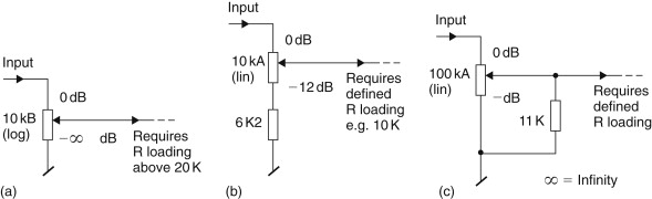
These considerations are true for ordinary pots with an audio taper, that is, those marked ‘log’ or ‘B’. As shown wired in Figure 8.9(a), these normally sweep over the maximum possible range of level setting, from a purely nominal 2∞ (hard CCW or “shut off,” really more like –60 to –70 dB) up to 0 dB (maximum level). The “audio taper” alias logarithmic resistance change per ° rotation makes the change in sound level reasonably constant with rotation. The full span and audio taper are relevant when a pot is needed to act sometimes as volume control, where output levels very much lower than the power amplifier’s capability are useful. It’s also relevant where a quick sweep to 2∞ (infinite attenuation) may be needed as a mute—to turn off the signal in one speaker, say—without switching off or unplugging anything.

Figure 8.9.

8.6.1.4. The Right Range

In many applications, the range offered by a raw pot is far too wide. In other industries employing pots, a vernier or a multiturn mechanism is added between the knob and shaft to aid fine settings. However, these are eschewed by modem professional audio operators, partly because of an ingrained fear of the loss of instant sweep control and because of relatively high cost versus relative fragility. There is also the false sense of alignment suggested by the verniers’ 3 or 4 figure scale; scales on different amplifiers would be strictly incomparable, owing to most pots’ poor tolerances, particularly good-sounding log pots. In the past 20 years, variations of 5 to 25% (or 0.5 dB to 3 dB) have remained the norm for the resistance mismatch between different pots at the same mechanical setting.

8.6.1.5. Linear Variants

Using a linear (A) pot and a fixed resistor, Figure 8.9(b) shows how adjustment range is restricted to the “top” 12 dB, that is, 0 dB to –12 dB. For system adjustment, this may be more usefully expressed as +/–6 dB. This range of adjustment is preferable for active crossover-based and arrayed systems, where the gain of individual amplifiers benefits from close adjustments and only needs this limited range. In practice, switched (say) –20 dB and 2∞ settings are then required. Note that the impedance vs. rotation relation is naturally slightly changed—the highest source impedance is here less at about 20% (rather than 25%) of the pot.

Returning to the full-scale mode, a linear pot may alternatively be used [Figure 8.9(c)], with a fixed resistor used for “law faking.” This converts the linear law to a log-like curve, if the pot and resistor values are kept within tight limits; this approach can give approximations of an audio taper that are at least more consistent than most log pots, which are made by butting n different-valued linear track segments together. Note that the pot’s effective value is here a tenth of its rated value after the law faking resistor is included. As a result, the pot shown in Figure 8.9(c) looks like a 10 kf2 pot to the load. However, the maximum source resistance is, as with the audio taper, at the 50% attenuation point and is just about 10% from maximum.

8.6.1.6. Position

As in other analogue audio circuits, the placement of any gain control device requires careful considerations in regard to considering trade-offs in headroom and SNR. But in power amplifiers having a minimum path, there is not much choice for location. They all end up after the input is unbalanced but before it is raised far.

Placement couldn’t be contemplated after the point of signal passing to the input of the power stage, for example, as pots having film tracks (cf. wire wound) that are suitable for audio by virtue of low rotation noise are unsuited to high dissipation. In any event, most power stage topologies don’t have a place for inserting a single-ended, passive voltage divider, don’t like having their gain widely changed, and are moreover wrapped around by NFB.

Adequate CMR (at the amplifier’s input) demands good balancing, which in turn relies on resistance matching to better than at least 0.5%, and since even makers of very expensive, high specification pots have problems maintaining matching between two or more sections to even 2%, over the entire travel, pots passing audio have to be placed after the input signal has been converted to single ended, that is, after the debalancer (DTSEC). Virtually all power amplifier gain pots (or whatever other gain control devices) end up thusly sandwiched. A few are used in active mode, where the pot is used in the NFB loop, of either an added line-level stage or even a gain-change tolerant power stage. This seems smart but it has its own problems.

Figure 8.10. Gain pot settings. Shown are six ways of looking at any power amplifier’s gain control; in this instance the simplest and most familiar “volume” control type. The final knob labeled “input clip volts (pk)” scale is for peak levels and is correct only for an amplifier that clips at 900 mV rms. In reality, the point would depend on speaker loading, mains voltage, the program, etc. The constant 9.6-V peak reached at lower levels shows where the input stage clips or where zener-based input-protection clamping is operating. Courtesy of Citronic Ltd.

8.6.1.7. Fixed Install

In amps principally intended for fixed installation, whether for a home cinema or public venues, and where power amplifier gain trims are needed or helpful for setting up, “knobless” gain controls are welcomed. Here, shafts are normally recessed and can only be turned with a screwdriver. This avoids not just casual tampering, but knobs being moved (and settings lost) by accidental brushing, sweeping, or knocking. A collet nut may be included. When tightened, the setting will then be immune to attack by a screwdriver, as well as vibration creep. As a further discouragement to “let’s turn this up,” such controls may be placed on the rear panel of the amp or hidden behind cover plates.

8.6.2. Remotable Gain Controls (Machine Control)

Pots are mostly made to interface with human fingers via knobs. When a sound system moves past the point where a single driver in each band can handle the power required or where Ambisonic or other multichannel sound is contemplated, remote control opens the door to “intelligent” control of loudspeaker systems and clusters, including balancing and tweaking directivity, imaging, and focusing, by machines and via wires and radio links. The gain of an amp can be controlled by a variety of electronic means (Figure 8.11). The purely electronic means are fast enough to perform additional, true processing functions, for example, limiting.

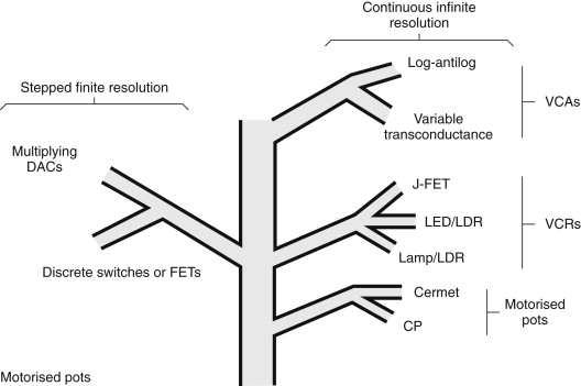
Figure 8.11. The family tree of electronically controllable gain and attenuation devices.

Usually a motor connects to the same shaft as a knob, but the latter via a slipping clutch. Either may override. This keeps the simplicity but shares the wide setting tolerance, sonic, and some of the mechanical limitations, of ordinary pots, for example, fragile shaft, relatively low setting speed. Which overrides the other depends on which way confidence most leans—toward human fingers or computers! Control circuitry is needed to decode remote command signals, which may be a variety of formats. Special driver ICs (e.g., BA series made by Rohm in Japan) make design and manufacture easy but might pose major replacement headaches to some owners in the future.

8.6.2.1. Voltage-Controlled Amplifiers

Commonly called a voltage-controlled amplifier, most are used as VC attenuators, usually as a solid state and always an analogue circuit. Most are ICs based around one of a limited number of proprietary schemes, which are made (or licensed, e.g., That Corp. in U.S. licenses, National in Japan) by one of three main patent holders, all in the United States.^[14] Otherwise they are based on a discrete circuit or on a consumer grade ‘OTA’ IC. Gain is accurately settable to within a fraction a dB, down to at least –70 dB and even into positive gain with some parts. Gain is always defined by an analogue control voltage (or current) that may be derived locally after decoding from a digital line or buss. Refined VCAs introduce considerable added circuitry into the signal path, which may defeat its own purpose. The simplest parts add two stages. They may boast low noise but it is at the expense of exposing the unnatural distortion patterns they create. The best performers add as many as five sequential stages and more than 5 op-amps may be required. If part quality is not to be compromised, the added cost seems high. Operating speed with most types can be very high, under 1 ItS. In this way, VCAs and all the following contrivances are applicable to dynamic functions, up to the fastest meaningful audio peak limiting.

8.6.2.2. LED+LDRs

With this method, the control signal drives an LED so that full brightness is defined as either maximum level or full attenuation. An adjacent light-dependent resistor (LDR) acts as the upper or lower arm of a passive attenuator. The intrinsic circuit isolation and physical separation that is possible makes LED/LDRs attractive in systems where isolation (of both grounds and common-mode voltages to 2.5 kV or more) is important for safety or EMC. These parts provide remote control connections analogous to connecting digital feeds via opto-isolators.

Tolerance is an issue and is dependent on the constituent parts, both semiconductors. Because the tolerance of both LDRs and LEDs is rather wide, manufactured combination devices are likewise broadly specified. The performance of both devices also varies widely with temperature. Also, in many circuits, there is no negative feedback loop to keep these variables within limits. Thus LDR/LED combinations are unsuited to system gain control due to inconsistencies of say +/–3 dB. They are fast enough to be used as limiters for bass and even midfrequencies in active crossover systems, and sonic quality is regarded as among the best. However, the above gain variation (in a population) would translate as a spectral imbalance, making overdriven conditions in a large system unsafe and/or uncomfortable, as well as drawing attention to the limiter action.

An LDR may also be partnered with an incandescent lamp. Even if small, the lamp is relatively slow to turn on and off, preventing its use for clean-cut dynamics processing, and lamp life span is more vibration sensitive and so not as certain as solid-state parts in road-going use.

8.6.2.3. Junction Field-Effect Transistors

JFETs are the lowest cost elements and can be made operative with little support circuitry. They are normally applied in the lower arm of an attenuator network. Without introducing complications of increased noise, noise pick-up, and other sonic degradation caused by introducing high ohmic value series resistors, attenuation is limited in range, and unless added circuitry can be justified, mild attenuation (around –6 dB) produces high (1 to 10% but mainly benign, low order) harmonic distortion.^[15] Low distortion control can be attained by placing the JFET in a control loop, comprising two or more op-amps and other active parts. However, as most JFETs’ R^on is in the order of a few tens of ohms, attenuation is still typically limited to –20 to –30 dB, enough for limiting, but not as a VCA gain and mute control.

8.6.2.4 Multiplying Digital-to-Analogue Converters

Multiplying digital-to-analogue converters (M-DACs) involve a resistive ladder, usually binary, with semiconductor switches, usually small-signal MOSFETs. They are the solid-state equivalent of a relay-controlled attenuator ladder (see later). Types suitable for high-performance audio must have dB steps—awkward in binary format—and special MOSFETs for low distortion and absence of “zipper” noise. The latter undesired sonic effect occurs in low-grade M-DACs; it is caused by step changes in DC levels or feed through from the digital control signal. Unlike the previous elements, an M-DAC has discrete resolution—just like a stepped (“detented”) pot. At low attenuations, step size must be no more than l dB for precise control; below –30 dB, larger steps (2 dB) are usually fine enough. To attenuate down to –70 dB in l-dB steps, 12-bit M-DAC is required.

8.6.2.5 R&R Array

Comprising resistors and relays, this is the mechanical counterpart of the M-DAC, with relays opening and closing paths in a “ladder” or other array of (usually) discrete attenuator resistors. Only high reliability, ATE-grade, sealed reed relays are suited for high-performance audio on grounds of both reliability and sonics. Such relays can act in under l mS and have fast settling, but are still not really suited to dynamics processing! Getting dB steps to act binarily with a resistor array takes some lateral thinking. Although the relays required are relatively expensive, by ingenious network adaptation to increment in binary dB, a mere seven can offer a 60-dB range in I-dB steps. With suitably well-specified resistors, this type can offer the highest transparency of any gain control device.

8.6.2.6. Summary

Motorized pots, lamp+LDRs, and relay/resistor arrays are good for remote- or machine-controlled gain trim and setting. The latter are the fastest and likely most reliable.

J-FETs and LED+LDRs are good for dynamics processing, but attaining accurate, noninvasive performance takes from the initial simplicity.

VCAs and M-DACs are elements that can do both kinds of jobs well.

8.6.3. Remote Control Considerations

Computers regularly feign precision that is only virtual. Until gain control elements become self-checking, self-calibrating, and self-aligning, they require careful specification.

8.6.3.1. Temperature

Pots (particularly conductive plastic), JFET, LDR, and particularly VCA elements are quite temperature sensitive. Unless designed with very low tempco, then when used in two or more channel amplifiers, they must be placed isothermally, that is, cosited to be independent of all the major temperature gradients, dependent on drive patterns, siting and even amplifier and rack orientation, as a hot gas usually rises upwards relative to the earth’s surface. This is true even with amplifiers employing forced venting, when small signal parts are not in an air path and are left to cool by microconvection, conduction, and reradiation.

Without such precautions, differences in channel gains of 2 dB have been observed in an amplifier employing VCA-controlled gain when driven up to working temperatures. This is enough to cause howl round or upset spectral balance.

8.6.3.2. Repeatability

Remote gain settings must not drift or have repeatability errors, which can accumulate to cause more than (say) +/–0.15-dB total error. This may seem stringent, yet on top of an initial tolerance of another +/–0.15 dB, it allows a worst case total difference between speakers of 0.6 dB. Other errors (cable losses, driver mismatches) are of a similar order and add to the differencing toll so there is no room for complacency. Least is best.

8.6.3.3. Conclusion

M-DACs and relay-resistor-array attenuators have the highest stability against temperature and time. Other types may prove acceptable with ameliorative engineering. Setting precision should not be taken for granted.

8.6.4. Compression and Limiting

Compression and limiting (comp-lim) are gain reduction, alias dynamics processing techniques, that are employed (among other things) to protect speakers, ears, and amplifiers from excess, distorted signal levels. In professional, active crossover-based systems, they are usually embodied within the active crossover. This is the best position for logistics in traditional large systems, with only one comp-limper band to worry about. Positioned within the filter chain can also be the best location for sonics.

Where power amplifiers are driven full range or where active crossover filter sections are integral to the power stage, compression and limiting functions may take place within individual power amplifiers.

Compression must be used sparingly, as average power dissipation in the drivers will be increased, potentially part-defeating the object, as speakers may then suffer burnout. Paradoxically, the compression threshold (at least for bass frequencies) should be increased if the gain reduction exceeds about 6 dB. Also, attack and release times require careful setting to avoid pumping on strong low bass.

Limiting is a higher ratio, more brute force (many dB-to- l) gain reduction. Its raison d’etre is to catch fast peaks, hence “peak limiting.” Attack times that are useful for protecting most loudspeaker drivers are in the order of 10 μS. Faster rising peaks that “get through” rarely cause damage to hardware, but may be reproduced efficiently by metal-diaphragmed drive units (cf. paper cones) and perceived and found highly unpleasant by the ear. Hence faster-acting peak limiters may enhance sound quality under many real conditions of “operator abuse.”

8.6.5. Clipping (Overload) Considerations

Driving any power amplifier with excessive input results in clipping because the output’s excursion is finite. Amplifiers offering higher power into a given load impedance provide a higher voltage swing into that impedance so clipping for a given sound pressure level is less likely to arise. However, linear increases in power give only underproportionate, logarithmic increases in headroom (in dB) and cost linearly ascending amounts of money. At some point, whatever more swing could be afforded would make no difference, and a limit is set. Exceeding this is clipping. For short periods it can be benign but else it is unpleasant and potentially damaging to hearing and positively damaging to hf and bass drive units in particular. Moreover, considerable overdriving, into hard clip, as can happen at any time by accident, even with domestic systems, can heavily saturate and thus vaporize the BJT output stages of inadequately designed power amplifiers.

8.6.6. Clip Prevention

Destructive and antisocial clipping may be prevented with comparatively simple circuits performing like a dedicated, fast limiter. There are as many names as there are makers. Some examples are shown in Table 8.6.

Table 8.6.

ARX systems	Anticlip
Carver	Clipping eliminator
Crest Audio	IGM (Instantaneous Gain Modulation)
Crown (Amcron)	AGC in PSA2 (Automatic Gain Control)
Malcolm Hill	Headlok

In these and related schemes, clip prevention does not occur until a dB or so of clip. Using the 100-W analogy, the usual low % THD does not rise until the signal passes above about 50 to 70 W. If headroom is adequate, this point should hardly ever be reached with the majority of recorded sound. With live sound, it may be reached quite often, but the fact that the deeply unpleasant point only l dB higher is not crashed through is of far more importance.

8.6.7. Soft Clip

“Soft clip” is a feature that aims to defeat the suddenness of the onset of hard distortion above the clip level in conventional, high NFB power amplifiers. It may be provided as a fixed or switchable option. Unlike compression and limiting, there are no time constants, no settings, and no attempt to avert serious distortion of a sine wave. However, the clipped waveform does not readily square off and retains some curvature (dV/dt) even with heavy overdrive (e.g., at +10 dBvr). This greatly reduces the massed production of unpleasant, high harmonics and intermodulation products of hard clipping. One apparent (but not necessarily actual) snag is that because hard clipping is a real limit, soft clipping has to begin to occur up to –10 dB below full output (–10 dBvr). This is tantamount to saying that distortion (%THD say) with a 100-W amplifier begins rising from above about 10 W, as opposed to rising very abruptly above exactly 100 W, while remaining extremely low up to this point. Here is one difference between low and high global feedback amplifier behavior.

Soft clipping restores the more forgiving behavior of low feedback to a high NFB amplifier. The extent to which it undoes all the high feedback’s other benefits is unqualified. At least the high NFB is in operation for most of the time, for with proper headroom allowance, most of the musical content should lie below the –10-dB threshold or so, whence the soft clip is inactive. Usually soft clipping is arranged to be symmetrical. This may not create the most consonant harmonic structure. Figure 8.12 shows a classic circuit.

Figure 8.12. A typical soft clip circuit as used in the Otis Power Station amplifier. Copyright Mead & Co. 1988.

8.7. Computer Control

Computer control of audio power amplifiers has been slow to develop. This is because amplifiers have not been a useful place, in most instances, for physical control surfaces. With a virtual control surface, the traditional limitation vanishes. In turn, installation setup, constant awareness of status, and troubleshooting of amplifiers in medium to large installations are all enhanced. One person can “be in six places at once.”

The Dutch PA system manufacturer Stage Accompany was a pioneer of the computer-controlled and monitored PA system in the mid-1980s. However, the first widespread commercial system that wasn’t a dedicated, integrated type was Crown’s IQ, running on Apple Macintosh (1986). The second was Crest Audio’s aptly named Nexsys, running on PC. Most subsequent systems have been IBM-PC-compatible types, running under Microsoft’s Windows. Every system is different, yet offers similar, fairly predictable features; there is no clear-cut choice. At the time of writing (1996), some “future proofed” universal, nonpartisan, networkable system contenders that seem most likely to become industry standards appear to have priced themselves out of consideration. Instead, makers continue rolling their own. Recent examples include the IA (intelligent Amplifier) system by C-Audio, the MIDl-based interface used by MC 2 (UK), and QSC’s Dataport system.

Today’s computer-control systems theoretically offer:

1. the remote control of many of most of the facilities and controls considered here and in other chapters.
2. the flexible ganging, nesting, and prioritization of these controls.
3. the transmission of real-time signal, thermal, rail voltage, or PSU energy storage data, monitoring, logging, and alarming. May even include a measure of utilization, for example, if a particular amplifier’s swing is largely unused as a consequence of overspecification.
4. the remote, even automatic, testing of amplifiers, speaker loads, and their connections.

Thus far, most computer-controlled power amplifiers require an interfacing card to be plugged in. Some types have integral microprocessors.

A well-designed computer control interface must not affect the analogue systems grounding or compromise mains safety. These requirements are met by the fiber-optic, opto-, or transformer-coupled interfacing, familiar enough in digital audio. Such systems must also not only meet EMC requirements, but also, in real world conditions, not radiate or introduce EMI to the power amplifiers. The system must also be able to recognize faults in its own connectivity to power amplifiers.