
A worksheet is a spacious place-16 billion or so cells at your disposal, each one accessible in a flash at the tap of a keyboard. The Name Box is your Excel—based satnav; type any address therein and the Box doesn't tell you how to get there—it takes you there, in a hot second.
But in spite all of that digital terra firma and ease of navigation, Excel gives you more, three worksheets by default, so you won't have to feel deprived—not with those 48 billion cells at the ready. But if even you don't need 48 billion cells, you might need three—or more—worksheets. Because while it's true that virtually all of the work you need to do in a workbook could be accommodated by one worksheet, sometimes it's the way data are organized in a workbook that make the multi-sheet approach a good idea, apart from any need for space.
For example, you may want to draw up a chart, or several charts, in a workbook, and keep them at arm's length from the data that gave rise to them (even though by default Excel places a chart on the same sheet as the contributing data, a decision you may want to override. However, Excel does assign pivot tables to a new sheet by default, as you'll see in the next chapter). That's a presentational decision, which could be motivated by a wish not to clutter the same sheet with a profusion of numbers and graphic objects. Or you may have a small business in which you want to earmark similarly-structured worksheets for each of your employees, with the same kinds of information about each assigned to the same cells on each sheet. (Remember that each worksheet has the same set of cell address—they all have an A45 or a LR5421, for example. How these addresses can thus be distinguished from one another is coming up soon.) Or you may want to store very different kinds of tables and the like on different sheets, should you need to dramatically redesign one of them and not impact the others. Or put more generally, your workbook may simply look better by placing disparate data in different sheets. More subtly, keeping a large collection of data on the same sheet could entail lots of scrolling up, down, and across the sheet, and as a result it might simply be easier to farm out some data to the upper rows of different sheets.
And even if you do disperse the data across several sheets, you can write formulas that reference cells on different sheets at the same time, a kind of three-dimensional way of working.
And in reality, I've badly undersold Excel's worksheet capabilities. If you wish, you can add worksheets to a workbook if events require, though on the other hand you can also delete two of the default three sheets, if you want to downsize your workbook. Finally, if your workbook needs are large, you can change Excel's default worksheet allotment, so that every new workbook starts you off with say, five new sheets.
In fact there's more to all this. Even before you begin to add more worksheets to your workbook, you can in effect enlarge the sheets you already have—by adding columns, rows, and even a few cells to existing sheets. Let's start by looking at this subject.
Having the capability to add rows, columns, and cells raises the obvious question: if you have all those billions of cells to begin with, why would you need to supplement them with even more? The answer—or at least the standard answer—is that after you've constructed a table, for instance, you may decide you need an extra field's worth of data—and that decision means you'll have to introduce a new column into the table. And if you want that column to appear between two columns already in place, you'll need to insert another one. If, on the other hand, you've entered data all over the worksheet and you'd like to see them a bit closer to one another, you may want to delete a column or two.
The means for adding and deleting columns or rows are pretty easy (although as usual, there's more than one way. We're demonstrating the most straightforward approach here). But before we demonstrate how it's done, we need to anticipate and answer a big question—namely, what happens to cell references when additions or deletions are carried out?
For example, suppose you've written this formula in cell H3:
=AVERAGE(B17:B32)
If you delete any of columns between C and H, will the cells referred to in that expression change? After all, delete one such column and the formula now appears in cell G3-and as a result, will the formula read
=AVERAGE(A17:A32) ?
The answer is no. When you add or delete rows or columns, Excel maintains the existing cell references that might otherwise be impacted by the additions or deletions, so not to worry. But keep in mind that if you insert a row or column such that cells contributing to a formula are repositioned, the formula will rewrite itself correspondingly. If a column is added to the left of the B column in the first example above, the formula will now read
=AVERAGE(C17:C32)
Because the values being added are now in column C.
To go ahead and insert a column, just click anywhere in the column to the right of where you want the new one to be inserted. Thus if you want to insert a column between H and I, click any cell in I. Then click Home

The new column will slide into place, and will claim the column letter I. The original column I will move to the right, and become J, and so on. If you want to insert multiple columns, just drag across as many consecutive columns as you wish and execute the above conmands. You'll insert as many columns as you've selected—and they'll appear to the right of the selection. Thus if you select cells R3:S3 and click Insert Sheet Columns, R and S will become T and U—because each will have moved two columns rightward.
The procedure for inserting rows is basically identical. Click in the row beneath which you want to insert a new one and click the above commands, culminating with Insert Sheet Rows instead. Thus if you click in row 17, you'll insert a new row above the original 17— which becomes the "new" row 17, whilst the original row 17 is now bumped to 18. To insert multiple rows select as many rows as you wish to insert.
To delete rows or columns, click anywhere in the column or columns you wish to delete and click Home
You can also insert and delete selected cells, not just entire rows and columns, a possibility which is curiously piecemeal. If you click in cell A12 and carry out the Insert Cells command, you'll push A12 down a row-but you won't push down row 12 in its entirety. Only the A column will be affected by the command. Any data in cell B12 will remain there, for example.
To insert or delete cells, click in the cell or cells in question and click either the Insert or Delete buttons we described in the previous to command sequences, but click Insert Cells... or Delete Cells... instead. Click Insert Cells and you'll see (Figure 7-2):

Click OK. If you select Shift cells right, all the cells to the right of the cell(s) in which you click will move in that direction—but not the cells to their left. The other two options you see—Entire row and Entire column—are nothing but alternatives to the Insert Row and Columns commands we've already described.
To delete selected cells, click in the cells you wish to delete and click Delete Cells... in the Cells button group (Figure7-3).

Note here that deleted cells move the remaining cells that are to their right to the left, and cells beneath them will be shifted up.
You can also hide rows and columns—not so much in order to maintain the secrecy of your data, but to improve the appearance of a spreadsheet; perhaps columns with complex formulas don't need to be seen—but if you do hide them, all the data posted there remain active, and any cell references to them remain in force, too.
To start hiding, click on any cell or cells in a column or row you wish to hide and click Home
Click and the rows or columns will disappear, as will the column letters and/or row numbers of the hidden items. To hide several rows or columns at the same time, just drag across those columns or drag down those rows, leave that selection in place, and click the commands you see in 7-4.
Now sooner or later you may want to reveal these clandestine areas of the workbook—and to do so you need to select rows or columns on either side of the hidden ones. For example, if the K column is hidden, just drag across any row in the J and L columns (e.g., J23:L23), leave that selection in place, and click the command sequence as per Figure 7-4—only here you'll click either Unhide Rows, or in our case Unhide Columns.
Now on to multiple worksheets, because extra space on your single worksheet may not be what you want.
As you can see, the three start-off worksheets that stock an Excel workbook share the same first name—Sheet1, Sheet2, and Sheet3 (you move between worksheets simply by clicking the tab of the sheet you want to access, or by utilizing these keyboard equivalents: Ctrl+Pg Dn to advance to the next sheet on the right; Ctrl+Pg Up to the next sheet to your left). But as with file names, Sheet1, etc. are default identities which can be changed as your needs require. As a result, you might very well want to rename any or all of these, and it's easy to do so. To rename a worksheet:
Right-click the tab of the sheet you want to rename. Click Rename on the shortcut menu (Figure 7-5):
Since the current tab is selected, just type the new name, and press Enter.

You can also rename the sheet by double-clicking the sheet tab in question, which also selects the tab. Type the new name and press Enter. You're allotted 31 characters per name.
Inserting a new worksheet is most easy, too. Just:
Right-click the sheet to the right of which you want to insert the sheet. You'll see again (Figure 7-6):
Click Insert.... In the Insert dialog box. The new worksheet will be selected by default.

Click OK. The new sheet appears, bearing the default name Sheet4, if it's the first new sheet you've inserted. And there's a still easier way to insert a new sheet. Click the Insert Worksheet button to the immediate right of the worksheet tabs (Figure 7-7):

Note the keyboard equivalent, too—Shift-F11. Clicking Insert Worksheet inserts a new sheet to the immediate right of the last sheet. It's the swiftest way to introduce a new sheet, but because it automatically installs the sheet at the end of the worksheet queue, you may decide you want to reposition the new sheet somewhere else.
Deleting an existing sheet entails right-clicking a sheet tab, then clicking Delete, and if it's empty, the sheet simply disappears. If the sheet contains data, this message materializes on screen (Figure 7-8):

Note that prompt. The word "permanently" means that if you click Delete, the sheet (and not just its data, in spite of what the prompt states) will not be retrievable via the Undo command. As a result, if you've accidently deleted a sheet you still need, you may have to resort to the classic close-the-file-without-saving-it technique. Don't say you weren't warned.
To continue our medley of right-click options: If you want to move or copy a sheet, either within the existing workbook or to another open workbook, or sheets (we'll soon see how to select multiple sheets), right-click the relevant sheet tab, and select Move or Copy....You'll see this dialog box (Figure 7-9):

As you see, you'll need to click on the name of the sheet before which you want the sheet to be moved. Note here that, by default, the To book: field names the workbook in which the sheet is currently positioned. If you want to move or copy the sheet to a different book, click the down arrow by "To book" to view the names of other open workbooks. Alternatively, you can click (move to end), whereupon the sheet will be resituated at the end of the sheet collection, no matter how many sheets you currently have on hand in the workbook. Then click OK.
Note that you can copy the sheet(s) to a different open workbook, too. Clicking Create a copy will do just that, replicating the sheet (including all its data) and placing it in the first position among the sheets (though obviously you can go ahead and move it). Copying a sheet coins a new sheet name based on the copied sheet, e.g., Sheet 2 (2).
Tip
You can also move a sheet by clicking the sheet tab (left button, this time), dragging it to its new position among the tabs, and releasing the mouse when you've reached your destination. A small page icon will accompany you as your drag, letting you know that sheet move is in progress.
And you can also recolor the sheet tab. Right-click the tab, select Tab Color, and select your hue from the resulting color selection. (Note: Your new color won't actually appear in the tab until you click on a different tab.)
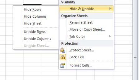
You can also hide entire worksheets, raising the obvious question as to why you'd want to. The principal reason isn't a desire to conceal the sheet from the dark intentions of industrial spies, covetous colleagues, or assorted other bad guys, because hidden worksheets can be revealed easily (there are Visual Basic programming means for securing the sheet with a password, though). Rather, you may want to hide a sheet because it contains complex formulas you'd rather not overwrite, or because all those calculations are unsightly (you can also protect all or part of a worksheet for much the same reasons, but protection options leave the sheet in view. More on protection a bit later.) Keep in mind that hidden worksheets remain active; that is, all their data and formulas continue to be available in the workbook, and can still be referenced by formulas in the visible sheets.
To hide a worksheet, right-click the sheet you want to hide and select Hide Worksheet. That's all. You can also execute the Hide command by clicking on the Home tab

Click OK, and the sheet reappears.
You can also group several worksheets, meaning that you can select them simultaneously. Why bother? Because by doing so, any data entry or formatting change you make in a range in one grouped sheet will be reproduced in precisely the same range in all the other grouped sheets, affording you a highly efficient way to achieve the same data arrangement and look across sheets. Thus if you enter a series of header rows in one grouped sheet—say, Name, Address, and Age—all those entries will appear in the same addresses on the other sheets.
To group sheets, click on the first one you want to group. You're then handed two group options: If you want to group non-adjacent sheets in a workbook, press Ctrl, leave that key down, and then click on the other sheets you want to group. Then release Ctrl. If you want to group adjacent sheets, click on the first tab you wish to group, then press Shift, leave that key down, and click on the last in the series of sheet tabs. To select all the sheets in the workbook, you can right-click any sheet tab and click b.
To demonstrate, open a new blank workbook and click the tab of Sheet1. Press Shift and at the same time click the Sheet3 tab (yes; you could have also clicked Select All Sheets, as per the instructions in the last paragraph). All three tabs should appear white (or at least whiter than usual, in the event you've colored any tabs), with the tab text "Sheet 1" appearing in boldface, indicating it is the active sheet. Then in cell A1 type Name, then Address and Age in cells B1 and C1, respectively. Then click Sheets 2 and 3—and you'll see the same data in the same cells. To deselect, or ungroup, the sheets, right-click any tab and click Ungroup Sheets (another dorky verb), or click on any sheet that is not currently grouped.
Now what about those multi-sheet cell references? As stated earlier, you can write formulas in which cells in different worksheets contribute to that formula result. For example, if you allocate a separate worksheet to each of three employees and enter their salary in the same cell on each sheet—say cell A7—you can write a sum formula, anywhere, on any sheet, which totals the three salaries. (And in fact the salaries don't have to be entered in the same cell address on the respective sheets. They can be situated in any cells.)
But let's start with a simpler case—you want to add two numbers on different sheets:
On Sheet 1 type 56 in cell D12.
On Sheet 2 enter 48 in cell B3. (Remember that the formula referencing these two cells can be written on any sheet—even Sheet 3, but we'll enter ther formula on Sheet 1.)
Click back on Sheet 1, onto cell A21. Once there, type the usual, and necessary, = sign.
Click on cell D12, the cell in Sheet 1 containing 56. You'll see:
=D12
Nothing new so far. Then:
Type the + sign, simply because we're about to add the contents of two cells.
Click the Sheet 2 tab, and click on cell B3. You'll see (Figure 7-11):

Note the budding expression in the formula bar: =D12+Sheet2!B3. By clicking on cell B3, the formula supplements that cell reference with the Sheet2! prefix, and why? Because, remember—we're actually writing this formula in cell A21 on Sheet 1, and so we need to indicate which cell B3 we're now referring to. After all, that cell could be in Sheet 1, Sheet 2, or Sheet 3—or any other sheet we might have inserted into the workbook. As a result, Sheet2! is Excel's way of notifying the formula that we want to call upon the B3 in Sheet2. Then press Enter, and we're snapped back to Sheet1, and the answer—104. And as with any Excel formula, its result will automatically recalculate, should either of its two contributing values—the 56 and the 48—be changed.
Now you may want to know why Sheet2! is attached to the second of the two cell references in the formula, but nothing like it accompanies the first. That's because the first cell reference-D12—appears in the same sheet as the one in which the formulawas written, and Excel assumes, by default, that unless the user indicates something to the contrary, all the cell references in a formula and the formula itself emanate from the same sheet—and after all, isn't that usually the case?
Now had we added these two numbers in a formula composed in Sheet3 instead—the sheet that contains neither of the values we wanted to add—we would have clicked in a cell on Sheet3, typed =, and then clicked on the two cells in Sheet1 and Sheet2 respectively. The formula would in this case have looked like this:
=Sheet1!D12+Sheet2!B3
See why? In this case neither cell shares its worksheet location with that of the formula itself, and so Excel needs to specify the worksheets on which both cells are positioned.
So that's the general approach to multi-sheet cell references in a formula—enter the = sign and the mathematical operation (or function) you wish to perform, and then click on the sheet and the cell(s) on that sheet you wish to incorporate into the expression. And if you need to reference a range of cells from another worksheet, you can just type = in your current destination cell, click on the first cell in the range on the sheet from which you wish to copy, then drag the appropriate range length, and press Enter. All those cells from the source worksheet are now referenced here, because they'll all be accompanied by the Sheet1, Sheet2, etc., identifier.
Now here's a neat variation on that theme. Suppose you want to add a group of cells, all of which have the same address in a collection of different worksheets—for example, values in the cell A3 in Sheets 1, 2, and 3. Let's try it:
In those three cells, enter 86, 72, and 4.
In cell C19 on Sheet1, enter =SUM(.
Then click on cell A3 in Sheet1, hold down the Shift key, and click on the Sheet3 tab.
You should see this in the formula bar:
=SUM('Sheet1:Sheet3!'A3)
Press Enter, and your answer—162—flashes into the cell (note you don't have to type the close parentheses. Pressing Enter automatically supplies it). With this technique, Excel automatically references the same cell in all the selected sheets—and by tapping the Shift key we've really grouped all three sheets (this method works with any Excel function, not just SUM. In fact, once you press Shift and click on the last of the sheets you want to reference, you can go ahead and drag any range you want. That range, with precisely the same coordinates, will be selected on all the sheets, and all will be calculated into the formula. Thus:
=AVERAGE('Sheet1:Sheet3!'A6:B14)
will calculate the average of all the values in the A6:A14 ranges on the three sheets.
Note in addition that a named range on one worksheet can be directly referenced on any other worksheet, without any concern for relative cell reference complications (note: this assumes the range's scope is the Workbook, which is the default in any case. See the Appendix on range names.) Understand a key point here-that the cell coordinates of a named range don't change—they're treated as absolute references (a point elaborated in the appendix) by default. Thus you can write:
=MAX(Scores)
But there's still another possibility: you can even reference cells in your formulas that come from other workbooks, that is, completely different Excel files. It's possible you'll need to calculate some bottom-line total for sales or budget data assigned to different workbooks, and have it all distilled into just one workbook; and that sort of task is eminently doable once the relevant cells are referenced. True, you'll want to proceed with care here, because if you email someone such a workbook—one containing cell references to data in another workbook—and you don't send along the latter workbook as well, your data will be missing something.
The way to go about referencing, or linking, data across workbooks is actually pretty easy, and similar to the method we described above for referencing cells across worksheets in the same workbook. Let's try this:
Open two new workbooks, and save one as Link, the other as Link2.
In cell G13 in Link type 65. In cell I2 in Link2 type 17. Now we're going to try and add the two numbers (needless to say, you can add many more than two, and you can link ranges as well this way).
Remaining in Link2, type =I2+ in cell A1.
Click on Link, and simply click cell G13. You'll see (Figure 7-12):
Then press Enter. The answer appears.

Note the syntax of the formula we've just written. Because we're working with cells in two different workbooks, Excel needs to specify two things: the workbook in which the linked cell(s) is located, as well as the worksheet, too. The name in brackets—[link.xslx]—obviously points to the workbook. Note as well that it's the cell that isn't in the same workbook as the formula that needs all these specifications, and note also that it's written with dollar signs, signifying an absolute reference. That's because if you copy the formula down a column, for example, Excel assumes you want all the copied formulas to reference the same cell in that other workbook.
Keep in mind that if you currently have only the workbook open that contains the linked cell and you change its data—and then later open the workbook containing the formula—the formula will recalculate automatically. And by the same token, let's say you change the data in the linked cell, close it and save it, thus leaving neither workbook open. When you open the formula-bearing workbook, it will likewise recalculate. (Note: If you move one of the workbooks to a different folder, the current link will be severed and will have to be reinstituted, if that's what you want, requiring a fairly messy repair job. An Edit Link dialog box appears, asking you to supply the new location of the moved workbook.) In sum, working with cell references can be a bit dicey, and should be used frugally. Apart from the moving-folder issue, tracking the cell references that contribute to your results can be daunting, particularly if you need to analyze a mistake in a formula.
I've said it before, and I'll say it again: workbooks are vast. You may have formulas scattered all across its worksheets, or even in far flung cells on the same sheet. And what if you've written a formula referencing cells in very different places on the workbook, such that when you changed the data in one such cell you could no longer see the new formula result on screen, because you've scrolled too far away? Well, you can always keep that result in your sights with the Watch Window option, located in the Formula Auditing button group in the Formulas tab. Let's try a very simple illustration, which should prove its point. Just watch.
Type 71 in cell D18 on Sheet1. Then type 21 in cell A2 in Sheet2. Return to Sheet1, and write the following formula in E17:
=D18+Sheet2!A2
Answer: 92. OK—been there, done that, got the t-shirt. But now click back onto Sheet2, and click Formulas

Then click Add Watch.... You'll see something like this (Figure 7-14):

I say "something like this," because the cell reference you actually see right now depends on the last cell you clicked on Sheet2, because that's where we are right now. But we want to track the current value of the formula in E17 on Sheet1, so just click that cell, and that reference should appear in the Add Watch dialog box. (Note: The dialog box asks you to click the cells you wish to watch, suggesting you could select a range. If you do, each cell in the range appears in the Watch Window, along with its value.) Then Click Add. You should see (Figure 7-15):

Note the dialog box records the workbook name as well as the sheet in which our watched cell is positioned; that tells you that if you have more than one workbook open at the same time, you can watch cells in any and all of them. The Name column, currently blank, is reserved for any range name you may have assigned a range you're watching (See Appendix XX). More obviously, the cell address and current value in the cell is recorded, along with the formula the cell is housing. Remember that we've clicked on Sheet2; so type 93 in cell A2, the cell on this sheet that is contributing to our formula. The Watch Window experiences a change in its Value column to 164—reflecting the new total in the formula in E17 on Sheet1—which we can't actually see right now. That's the point; the Watch Window keeps us posted of changes in the values of cells that, at the moment, aren't visually available to us. To turn off the Watch Window, just click the standard X in the window's upper-right corner. The Watch Window isn't remembered by the saved workbook. It has to be reconstructed if you want to use it again with a reopened workbook.
You'll recall that we earlier described how you can hide worksheets from view—an option that surely has its advantages, because the data on that reclusive sheet are gone but not forgotten. You can still refer to the data in formulas and the like, even as the sheet stays out of harm's way. But there's an obvious downside here: the sheet is...hidden, and while you may enjoy the security that worksheet invisibility affords, you may want to have your cake and eat it too—you may want to be able to view your worksheet data even as you fend off the errant mouse clicks that could obliterate your finely-tuned, guru-worthy formulas. Protecting your worksheets—either all or in part, by protecting just some of its cells—is the way to achieve those ends, and the how-tos are pretty simple and reasonably secure, if just a mite quirky.
When you protect a worksheet you can continue to see the sheet and its data, but once the protection is in force you won't be able to enter any additional data in its cells. You will, however, be able to view the underlying formulas in cells, and you will be able to copy the data you see in protected sheets. At least, that's how the default protection settings work. You can, however, also opt to hide formulas in their cells via protection. And in addition to protecting individual worksheets you can protect workbooks in their entirety (with different consequences, as we'll see), or protect just selected cells in a worksheet instead.
To protect a sheet, click in any cell, then you can either click:
Home tab
Review tab

If you click OK, the sheet will revert to protected status, with the default selections you see checked above put in place. And what do those selections mean? Select locked cells and Select unlocked cells mean that you'll be allowed to click on any cell in the worksheet—but you won't be able to enter any data in it. (It does mean, however, that you'll still be able to see any underlying formulas in any cells.) And what's a locked cell? I was afraid you'd ask that question. For starters, what it means is that if you check both of the above default options off, you won't even be able to click on any worksheet cell. And if you click only Select locked cells off, you'll be able to click on unlocked cells only.
But I still haven't defined locked cells—so here goes. By default, turning on worksheet protection locks all of a worksheet's cells. But if you want to able to enter data in just some cells and leave the remainder of the sheet protected, you have to inform Excel about this intention before you turn protection on (I told you it was quirky). If that's what you want to do—that is, be able to enter data in some cells only—then before turning protection on, first select those cells you want to leave available for data entry, and then click either the Home tab

Déjà vu? We're back to a dialog box we've seen a few million times before in previous chapters, but here you need to click the Protection tab, something we haven't yet done. Click it and you'll see (Figure 7-18):

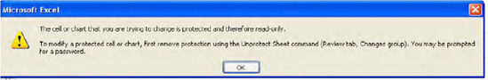
Then click Locked off and OK. Just remember the sequence of events: We want to be able to enter data in only certain cells on a worksheet, and at the same time protect the rest of the sheet. Start the process by selecting those cells that will remain available to data entry, and then call up the dialog box you see above and uncheck Locked. Then—and only then—can you go ahead and turn Protection on. That will do the job—and as a result, you'll be able to carry out normal data entry in the unlocked cells. If you attempt to type anything in a protected cell, though, you'll encounter this error message (Figure 7-19):
The prompt in Figure 7-19 informs you of one—but only one—way of returning the entire worksheet back to normal data entry status, or its unprotected state: Review tab
The whole process is curiously backwards, but it's always worked this way: select the cells in which you'll want to able to enter data, uncheck Locked in the Protection tab of the Format Cells dialog box, and then protect the worksheet. And once a cell is unlocked and you go on to protect the sheet, you can't click the Lock Cell option (see below in figure 7-15) to lock that cell back along with the rest of the sheet.
There is, however, another command out there—an alternative way to unlock cells before you protect a sheet—that may rank among Excel's most puzzling. If we return to the Cells

The problem with Lock Cell is that when you click it, it designates any cells you've selected to be unlocked if you go ahead and protect the worksheet. Don't ask questions—it's a toggle, an alternately on-off click result.
And what about that Hidden option offered up in the Format Cells
You also doubtless noted the password option featured in the Protect Sheet dialog box (Figure 7-21):

Entering a password prevents you—or anyone else—from unprotecting the sheet. Once you type a password—which is optional—another dialog box appears (Figure 7-22):

Note the caution. Once you click OK, the password is duly recorded. Try now to unprotect the sheet, and you'll be prompted for the password. Hope you wrote it down.
You can also protect an entire workbook—but doing so brings about a result you're not likely to expect. Protecting a workbook does not seal off every cell in the entire book from data entry. On the contrary; if you protect a workbook, all its cells can continue to receive data. Rather, workbook protection prevents the user from making what Excel calls structural changes in the book—that is, adding moving, renaming, or deleting worksheets. It will also allow you to protect against changes to current window sizes, meaning if you accept this option and your worksheet currently occupies less than a whole screen's worth of space, you won't be able to restore it to full size via the Maximize button, for example. But that's a less relevant option for most users.
To protect a workbook, click the Review tab
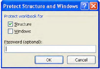
Note the dialog box isn't titled Protect Workbook, but that is what it's offering to do. And as you see, it's password controllable, and you'll be asked to confirm that password should you choose one. Click OK, and as stated earlier, you won't be able to reposition worksheets, change their names, or delete any of them. To turn Protect Workbook off, just click the Protect Workbook button again. If you've protected the workbook with a password, you'll be asked to supply it.
You may have constructed a workbook—or inherited one—in which similar data are compiled on separate worksheets, say, the sales totals compiled by a set of salespersons across a set of years, each year assigned its own worksheet. If you want to then combine these yearly totals into one summary worksheet, in order to see how much each salesperson has earned overall, you can use Excel's Consolidation tool to do the job.
To demonstrate how Consolidate works, download the Sales By Year workbook from www.apress.com. You'll see a small listing of salesperson data for the years 2008, 2009, and 2010. Note each sheet is identically organized—that is, the ordering of the salespersons is the same in each year, and each sheet's data column is headed Sales (remember that by grouping worksheets you can do this easily—entering labels in one grouped sheet reproduces those same labels in the same cells in the others). On each sheet name the range A4:B8 Sales08, Sales09, and Sales10, respectively (Figure 7-24):

Note in addition that a fourth sheet, containing the same labels but no data, is supplied as well. If you were consolidating your own sheets you'd need to draw up such a sheet, because this is the one on which the consolidated results will appear. Then to begin consolidating, select cells B5:B8 in the Consolidated Data sheet(Figure 7-25):
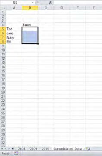
Figure 7.25. The Consolidated data sheet—marking out the range in which the consolidation results will appear
Then click the Data tab

The options presented here require a bit of explanation. You can carry out two kinds of consolidation—consolidation by position and consolidation by category. We're going to start with consolidation by position, which is the approach you'll take when the data labels on the various sheets are all in the same position, as they are in our sheets. Since our three sheets line up their labels in exactly the same way, all we need do in the Consolidate dialog box above is enter the ranges in which the data appear in the three yearly sheets. Click in the Reference field if necessary, and then click the 2008 tab, drag cells B5:B8, and click Add. You'll see (Figure 7-27):

Then click sheet 2009, select cells B5:B8, click Add, and do the same for sheet 2010. (Note that when you click on sheets 2009 and 2010 you should find that B5:B8 is already selected. If not, just drag those cells.) Then click OK in the above dialog box. You should see (Figure 7-28):
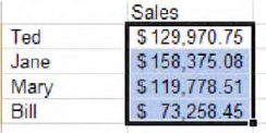
The data are consolidated in the Consolidated Data sheet. Each salesperson's sales totals for the years 2008-2010 are now recorded, or consolidated, in one cell. Again, this is a consequence of the data labels on the three yearly sheets all holding the same relative position. Thus Consolidate knows that because Ted is the first-listed salesperson on all three sheets, the first cells in the three ranges we added to the Consolidate dialog box all represent Ted's sales data, and so on. (Important note: Working by position, as we've done here, doesn't require that the salesperson's labels on the respective sheets all share exactly the same addresses. They need to share the same relative position, such that Ted would always be listed first, followed by Jane, etc.)
Now for what again is called consolidation by category. Delete the results in the Consolidated Data sheet (but not the data labels) and click on sheet 2008. Switch the positions of the names Ted and Jane, so that Jane is now listed above Ted. Then click back on the Consolidated Data sheet and this time select A4:B8, which includes the data labels—something we didn't need to do when we consolidated by position. Then click Data Tools
Then click the Top row and Left Column boxes in the Use Labels in area of the Consolidate dialog box, and click OK. You should see (Figure 7-29):

Note the totals here for Ted and Jane differ from our previous results because we've switched the positions of Ted and Jane's names, and hence their sales totals, in sheet 2008. We've just carried out a consolidation by category, in which the names of the salespersons don't share the same relative position across the three sheets. That's why we needed here to click on Top Row and Left Column to orient us, because Consolidate needs to "find" all the salespersons and their data by looking for their names and the Sales label on each sheet—wherever they may be positioned.
That point may call for a bit of review. "Consolidation by category" means that Excel will search for salespersons' names wherever they happened to be positioned on the 2008, 2009, and 2010 sheets. The salespersons are the categories here.
There's one other Consolidation option that you may want to explore—Create links to source data. Checking this enables you to change the numbers in any of the sheets contributing to the consolidation, such that those changes will be recorded in the consolidation result. To demonstrate, return to the Consolidated Data sheet and make sure range A4:B8 is selected, with the results you've seen above. Then click the Data tab
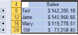
You'll note the obvious addition to the screen. A collection of plus signs has taken over a new, gray area to the left of the worksheet proper, and you'll note as well that the row numbers exhibit gaps in their sequence, and—less obviously—that a new third column has inserted itself between the salespersons' names and the actual sales data. Click one plus sign and you'll see (Figure 7-31):

You've viewing an instance of Excel's outlining capability, which in this case breaks out the three years' worth of sales data for Ted. Clicking the plus sign reveals—or expands—these data, which had been hidden—thus explaining the row-sequence gaps we noted earlier (you may also want to widen the columns so as to better view the Sales By Year labels). These new data really consist of cell references to the relevant data in the three yearly sheets for each salesperson. Thus by clicking the first such row for Ted, you'll see in the formula bar:
='2008'!$B6
which references the cell in sheet 2008 in which Ted's sales data appears. And because we're working with cell references, changing any data in these linked cells will change the consolidation result here. Then, clicking what is now a minus sign collapses these detail rows and hides them again. Click the 2 you'll see in the upper reaches of that gray area housing the plus-minus signs will expand all the hidden row data for all the salespersons, and clicking 1 collapses them (Figure 7-32):

And if you click the Data tab
And that's how to consolidate data across multiple worksheets. On the other hand, the consolidation options aren't terribly flexible, and you may decide that other alternatives to aggregating data, particularly pivot tables, will better suit your data gathering needs. And as it turns out, we're going to take a look at pivot tables in the next chapter.
Workbooks consist of worksheets, and those sheets can be treated as stand-alone objects that contain their own, independent data, or they can be connected in various ways to the other sheets. We've reviewed a batch of ways in which those connections can be made—either through cell references, grouping, or consolidation of their data. We've also seen how to protect the data on your sheets, either wholly or partially, on a cell-by-cell basis.
Just remember—you've been entrusted with the care and feeding of 16 billion cells. It's an awesome responsibility—so take good care of them.