
It's easy enough to understand how to identify a range – e.g., A34:R78 refers to all the cells camped out between A34 and R78, including those two cells which hold down the upper left and lower right corners of the range. But that reference isn't as informative as it could be. You might want or need to know what kind of data populates a range, be they test scores, income figures, or population statistics. As a result, Excel lets you name a range and use it in a formula, so that an expression such as
=SUM(A6:A20)
could be rewritten to read
=SUM(Income)
where the word "Income" represents or acts as a proxy for A6:A20, which could be listing a collection of income data. Naming a range helps you, and anyone else who may be viewing the workbook, to quickly understand what the range is about, and can also ease the formula writing process. After all, it may be simpler to type
=AVERAGE(tests)
than
=AVERAGE(B15:B112)
which requires you to remember those range coordinates, and/or drag down all those cells.
And there's another reason you might want to name a range, one I alluded to about 300 pages ago. I wrote there about naming a range which consists of exactly one cell. If that cell – say C1 - is applied repeatedly to different formulas – say a constant grade bonus of five points entered in that cell, added to a series of test scores listed down a column – I'd have to write something like
=A3+C$1
and then copy that formula down the column in order to add the five points to all the other exams listed down the A column. The dollar sign establishes an absolute reference, whereby the 1 in C1 is held constant. But if you name C1 Bonus, for example, you can write
=A3+Bonus
without having to worry about those dollar signs. Naming a range automatically holds its cell references constant, no matter where you copy it.
Naming a range is easy, although as usual Excel offers you more than one way to achieve this end.
In order to get the hang of this, first download the Range Names workbook from the book's page at www.apress.com. The simplest approach to range naming is to select the range you wish to name, click in the name box, type the name, and press Enter. Thus if you want to give a name to the range A6:A20, select those cells, click in the name box, type Income or any other name you wish, and tap Enter (Note: multi-word range names such as test scores must be joined by an underscore: test_scores. If you omit the underscore you'll trigger this error message: "You must enter a valid reference you want to go to, or type a valid name for the selection."
The latter half of that caution refers to range names, the first half, to the navigational role played by the name box we referred to in Chapter 2. It's perfectly legal to name a range with just one letter – a, or p, something equally spare – and while a one-lettered range name won't tell you too much about the range, it's obviously easy to apply to a formula. Note that your named ranges will be listed when you click the drop-down arrow alongside the name box; click any such name and Excel will immediately highlight that range on your workbook. (Figure A-1):

An alternative way to compose a range name is particularly apt when your range is topped by a named header row. Let's say cells A6:A20 feature a header named Income in cell A5. Select that A6:A20 (note that you need not select A5) and click the Formula tab

Click OK, and the range is named. Note the range does not include row A5, the row which contributed that name (as you can see, you could have entered a diferent name in the Name field, though doing so would have defeated the purpose of calling upon the header row. Excel decides on the range namehere by grabbing onto the label - Income – in the immediately preceding cell. Had a value been stored in A5 – well, Excel won't drum up a range name from there; you'll have to make one up yourself.
While we're at it, here are some other range naming rules:
Range names can contain up to 225 characters
They must begin with a letter
You can't define a name that resembles a cell reference, e.g., X345. X345Score is legal, though.
That last criterion needs to be refined a bit, and points up a subtle downside which besets named ranges. Because the pre-2007 releases of Excel were confined to 256 columns, it was permissible there to name a range XAA321, for example, because that name refers to a cell which doesn't exist in those versions. That same reference won't be accepted as a range name by Excel 2010, however – because cell XAA321 is a perfectly valid address in 2010.
Note also that you can use the Define Names dialog box to assign a name to a value. That is, you can enter a value in the Refers to field instead of cell coordinates, and the name you assign to that value can be used in formulas as well (Figure A-3):

The Scope field is a bit more obscure. Note that Workbook is set as the default scope-and that means that this range name can be deployed in any cell in the workbook without additional qualification. Thus if I name the range A6:A20 in Sheet 1 Income and leave the Workbook scope default in place, I can write a formula such as
=AVERAGE(Income)
in Sheet 2 as you see it above. If, however, I define the scope of A6:A20 as Sheet1, I'd have to write the above formula in Sheet 2 this way:
=AVERAGE(Sheet1!Income)
Obvious question, then: why bother to restrict the scope here to Sheet1? It requires more work to write formulas this way. The answer is that you may want to name a second range, this one in Sheet2, as Income too, and so you'd need to identify the particular sheet in any formula reference to distinguish between the two Income ranges However, if you do confine the scope of this formula to Sheet1, you can still write
=AVERAGE(Income)
in Sheet 1 itself. Write exactly the same expression in Sheet2 and it'll refer to that range in Sheet2.
The Comment field lets you enter a description of the range you're naming, thus explaining to other viewers of the workbook exactly what you had in mind using the name.
You'll also note that the Define Name command features a drop-down arrow. Click it and you'll see a rather quirky option, Apply Names. Apply Names lets you replace a standard range reference in a formula with its name, if you've devised that name after writing the formula. For example, if you've written
=AVERAGE(A6:A20)
in a cell and then named A6:A20 Income, you can click in any blank cell, click Define Name

The above formula will now read
=AVERAGE(Income)
And so if you've named five different ranges after you've already written formulas containing their actual cell references, you can click any blank cell, select Apply Names, click on all five range names in the Apply Names dialog box, and those names will replace the cell references in all the formulas. Yeah – that blank cell thing is quirky indeed.
As indicated, once you've named a range you can apply it to a formula. You can simply type, for example
=AVERAGE(Income)
Or you can start to write the formula, and when you get this far
=AVERAGE(
click the Use in Formula button in the Define Names button group. If you do, you'll see (Figure A-5):
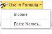
(Needless to say if you name several ranges, all of their names will appear in the drop-down menu.) Click Income and that name will be inserted into the formula. On the other hand, you could also starting typing
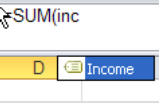
=SUM(Inc
at which point you'll see the name Income appear in the auto complete function menu (Figure A-6):
And once you click the Use in Formula button you'll likewise notice the Paste Names option, a slightly ambiguous one – because it suggests you can paste a range name into a formula. But we just did that, and without the assistance of this command. But Paste Names does two very different things. Clicking Paste Names activates a dialog box bearing two options – Paste List and OK. Clicking Paste List won't insert a range name into a formula – rather, it'll simply list the ranges you've named somewhere on the workbook, beginning in a cell of your choosing.
Let's say, for example, I've supplemented the Income range name with a second named range, called Staff, occupying cells K6:K12 and headed by the name Staff in K5. Click in cell E14 and click Paste Names (Figure A-7):

Click Paste List and you'll see (Figure A-8):

We see that indeed, the ranges are simply listed on the selected worksheet, in this case starting in E14 (and thus the screen shot above spans cells E14:F15) with both names and range coordinates reported. Paste List can be a handy means for keeping track of the whos whats and wheres of all your named ranges right there on a worksheet, without having to return to any dialog boxes to learn that infomation.
But click the OK button in the Paste Nanenes dialog box and you get something else entirely. If I click in cell B6, the cell to the right of the first income figure, and click Use in Formula

Press Enter and you'll see 34567 – the contents of cell A6. But the formula bar view for that cell will display =Income. What that means – at least what that means here – is that pasting the name of the range Income in B6 posts the data in the corresponding Income cell only – which is A6 in this case. If I copy the result in B6 down the B column, I'll return each corresponding value down the A column-even though each one of those cells will actually state =Income. You're reporting each individual value for each cell comprising the Income range – even though each of these cells is referenced by =Income – which of course stands for cells A6:A20 – the whole range. I know what you're thinking – this one is pretty quirky, too.
Thus clicking OK in Paste Names requires - before you click OK - that you click in cells which must line up with, or correspond to, the cells in the range name being pasted. If you carry out the Paste Name command sequence in cell B4, for example – a cell which does not correspond to any Income range cell in the A column – you'll see the #VALUE! error message in that cell after you press Enter.
The next option in the Defined Names button group – Create From Selection – dates back to Excel's antiquity. Click on the Bowling Scores sheet tab on the Range Names workbook and select cells F10:I15 – a range which contains a collection of bowling scores as well as name and game-number labels (and make sure you've selected the labels). Click Create From Selection, and you'll see (Figure A-10):

Click OK and nothing really seems to happen on screen. But click the down arrow by the name box (Figure A-11):

Something did happen. Excel has fashioned a range name for each row and column in the range you selected, by appointing the data in the top row and left column as respective range names. Click on Bob, for example, and Excel will highlight cells G11:I11 – those cells which appear to the immediate right of Bob's name. Thus Create from Selection is a fast way to assign range names to individual rows and columns of data, by grabbing onto labels that top each row and sidle each column. (Note, by the way, that the Game One, etc. labels were rewritten as Game_One, and so on, because range names cannot contain spaces.)
The final and largest button inlaid into the Defined Names button group is the Name Manager. Click it and you'll see (Figure A-12):
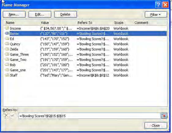
Most obviously, the Name Manager lists all the workbook's named ranges, identifying their location, some of the values populating the cells in the ranges, and their scope and any comments about the range. By clicking Edit after clicking on a range name you'll be brought to an Edit Name dialog box, which enables you to both change the range's name as well as the range's coordinates. Click on a range name and then clicking Delete will naturally delete the range's name – but not the data in its cells (you can also do the same by clicking on a name and tapping the delete key). Clicking the Name header sorts the ranges names in A-Z order.
The Filter button displays a list of options by which you can selectively view certain of your named ranges (Figure A-13):
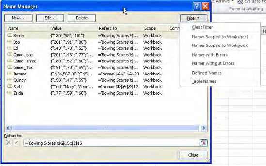
The Names with Errors filter option lists only those ranges containing any values which exhibit an error message, e.g., #REF or #VALUE!.
Range names can add a measure of ease-of-use to the formula writing process, and can inform the user—and her colleagues—about the contents of a range. On the other hand, there is a view that range names should be used with caution, as there's some evidence that they may hobble the spreadsheet error debugging process. Your decision to name ranges will depend, as usual, on the purposes you bring to your workbooks, and their complexity. But for straightforward formula writing tasks they're good to know about.